Atmospheric Kelvin–Helmholtz billows captured by the MU radar, lidars and a fish-eye camera

Abstract

On June 11, 2015, a train of large-amplitude Kelvin–Helmholtz (KH) billows was monitored by the Middle and Upper Atmosphere (MU) radar (Shigaraki MU Observatory, Japan) at the altitude of ~ 6.5 km. Four to five KH billows in formation and decay stages were observed for about 20 min at the height of a strong speed shear (> ~ 30 m s⁻¹km⁻¹), just a few hundred meters above a mid-level cloud base. The turbulent billows had a spacing of about 3.5–4.0 km (3.71 km in average) and an aspect ratio (depth/spacing) of ~ 0.3. The turbulence kinetic energy dissipation rate estimated was of the order of 10–50 ${\text{mWkg}}^{ - 1}$, corresponding to moderate turbulence according to ICAO (2010) classification. By chance, an upward-looking fish-eye camera producing pictures once every minute detected smooth protuberances at the cloud base caused by the KH billows so that comparisons of their characteristics could be made for the first time between the radar observations and the pictures. The main characteristics of the KH wave (horizontal wavelength, phase front direction and phase speed) obtained from the analysis of the pictures were fully consistent with those found from radar data. The pictures indicated that the billows were advected by the wind observed at the height of the critical level. They also revealed a very small transverse extent (about twice the horizontal spacing) suggesting that the large-amplitude KH billows were generated by a very localized source. Micro-pulse lidar and Raman–Rayleigh–Mie lidar data also collected during the event permitted us to confirm some of the characteristics of the billows.

Introduction

Shear flow instabilities leading to Kelvin–Helmholtz (KH) billows are quite common in the atmosphere. They are a principal source of mixing in stably stratified conditions and have therefore been studied extensively by using in situ and remote sensing techniques (e.g., Fukao et al. 2011 and references therein). Radars and lidars can provide excellent means for studying these phenomena, and large-amplitude KH billows have often been monitored by the VHF Middle and Upper Atmosphere (MU) radar (Shigaraki MU Observatory, Japan) (e.g., Luce et al. 2008). However, remote sensing measurements of KH billows are usually not confirmed by direct naked eye observations supporting their interpretations. Coincident observations are indeed difficult to obtain because KH billows either occur in clear air conditions so that they are invisible, or happen in association with clouds but not under conditions permitting us to make valuable comparisons. In addition, photographs from standard cameras are generally taken only if the opportunity arises, which is not easy to seize. In the present work, for the first time, characteristics of KH billows simultaneously captured by the MU radar and two lidars are described with observations made by a vertically pointing fish-eye camera. Radiosonde data are also available. The dataset was collected on June 11, 2015, during a multi-instrumental field campaign called ShUREX (Shigaraki UAV-Radar Experiment, Kantha et al. 2017). On that day, the conditions were ideal for concurrent observations because the KH billows were generated above a cloudy frontal layer at an altitude of ~ 6.5 km (about 1 km above the cloud bottom) and dry conditions were met down to the ground so that the camera and the lidars could probe the cloud base. The KH billows were confirmed by photographs taken once every minute by the fish-eye camera through disturbances they produced at the cloudy interface. In the camera images, these disturbances took the form of spanwise elongated protuberances organized in horizontal bands moving in time. Turbulence kinetic energy dissipation rates $\varepsilon$ associated with the KH billows corresponded to moderate turbulence for medium-sized aircrafts according to ICAO (2010) classification $(0.4 < \varepsilon^{1/3} < 0.7\,{\text{m}}^{2/3} {\text{s}}^{ - 1} )$.

The lidar data confirmed the roll-up of KH billows and the entrainment of condensed particles along the braids. Incidentally, the KH billows were accompanied by a mid-level cloud base turbulence (MCT) layer (Kudo et al. 2015) developing in the sub-cloud region a few tens of minutes prior to their appearance without evidence of relationship between the two events.

The collected datasets thus gave us the serendipitous opportunity to compare the properties of KH billows inferred from VHF radar and lidar observations and those obtained from a direct analysis of the fish-eye photographs. In meteorological applications, fish-eye camera photographs are commonly used for estimating cloud fraction, classifying cloud type and measuring the height of the cloud base (e.g., Long et al. 2006 and references therein). They have also been used in combination with remote sensing data such as lidar data for helping interpret the remote sensing observations of clouds (e.g., Sassen et al. 2003; Schultz et al. 2006). But, to our knowledge, it is the first time they are used in combination with VHF radar and lidar data for analyzing KH billows. The pictures also permitted us to get additional information on the horizontal extent of the KH billows and to reduce ambiguity on the interpretation of their Eulerian time evolution in the radar and lidar images.

In “Instrumental setup” section, the instruments are briefly described. “Analyses of the observation results” section shows the observation results and describes the characteristics of the KH billows from the cross-analysis of the radar, lidar, balloon and fish-eye camera data. Finally, conclusions are given in “Concluding remarks” section.

Instrumental setup

The MU radar is a pulsed VHF (46.5 MHz) Doppler radar located at the Shigaraki MU Observatory (34.85°N, 136.10°E), Japan (e.g., Fukao et al. 1990). In addition, the observatory also houses a micro-pulse lidar (MPL) and a Rayleigh–Raman–Mie (RRM) lidar, among other remote sensing instruments. It is also equipped to launch meteorological radiosondes. Finally, last but not least, for the present study, a fish-eye camera located on the roof of the building takes photographs of the sky overhead. Figure 1 shows the location of the instruments at the observatory.

Fig. 1

Photograph of the Shigaraki MU Observatory. The black dot and the vertical dashed line show the location and upward-looking direction of the fish-eye camera, respectively. The blue line shows the vertically pointing beam of the RRM lidar. The green line shows the MPL beam steered 30° off zenith toward north

The MU radar

The details of the radar parameters used during the campaign are shown in Table 1 of Kantha et al. (2017). The central vertical beam of the radar was operated in range imaging mode with five equally spaced frequencies from 46.0 to 47.0 MHz for high-resolution observations at vertical incidence (typically a few tens of meters), while the north, northeast, east, southeast and south beams, steered 10° off zenith, were operated in a standard mode of 150-m resolution for additional atmospheric parameters (such as horizontal winds). One vertical profile of parameters was estimated every ~ 4 s from time series of ~ 16 s in length (corresponding to a time overlapping of a factor 4). The high-resolution echo power images were obtained with the adaptive filter-bank Capon processing method (Palmer et al. 1999; Luce et al. 2001). As illustrated by, e.g., Luce et al. (2010) and Fukao et al. (2011), the range imaging mode enables atmospheric echo structures to be more clearly delineated and can provide a better understanding of the observed phenomena.

Table 1 KH billow characteristics from fish-eye camera photographs

The lidars

The micro-pulse lidar (MPL) is an autonomous laser radar system originally developed at the National Aeronautics and Space Administration’s (NASA) Goddard Space Flight Center (GSFC) (Spinhirne 1993). The MPL-4 system (Sigma Space Corporation, USA) operates at a wavelength of 527 nm. Data averaged over each 20 s were acquired with a 15-m range resolution. Because the telescope was steered 30° off zenith toward north during the observation period, the vertical resolution was approximately 13 m. The raw data were converted into relative backscatter using algorithms presented by Campbell et al. (2002).

The RRM lidar has a Nd:YAG pulsed laser (532 nm, 600 mJ, 50 Hz output) and a telescope of 82 cm in diameter. The received signals are divided into several channels for different measurements (two elastic channels, two rotational Raman channels and one water vapor Raman channel at 660 nm) (Behrendt et al. 2004). During the observation period, it was operated with time and range resolutions of 20 s and 7.5 m, respectively, at vertical incidence. The backscatter signals of elastic channels were employed for cloud observations.

The fish-eye camera

The camera is a PSW-100W2 Skyview all-sky camera (Prede Co., Ltd., Japan) and is programmed for shooting every minute. The images are stored to a PC as JPEG files. The fish-eye lens angle of view is 180° in all azimuths, and the projection method $y = 1.24 f\,\sin \left( {\theta /1.24} \right)$, where f is the focal length and $\theta$ is the zenith angle, permits us to retrieve the horizontal distances y. A shading blade to block off direct sunlight rotates automatically to track the solar orientation, which was calculated from observation time, longitude and latitude.

The Vaisala Radiosonde

A Vaisala RS92G Radiosonde was released from the radar site at 0706 LT on June 11, 2015, and provided vertical profiles of pressure, temperature, relative humidity and zonal and meridional wind components, u and v, at a frequency rate of 1 Hz (corresponding to a vertical sampling of ~ 5 m). From these data, it is possible to retrieve vertical profiles of potential temperatures and atmospheric stability parameters.

Analyses of the observation results

Radar and balloon data

Figure 2 shows the time–height cross section of high-resolution radar echo power (in dB, arbitrary units) at vertical incidence between 0600 LT and 0800 LT on June 11, 2015, and in the height range 1.27–8.00 km. The image essentially reveals two distinct regions separated by a layer of enhanced echo power appearing and thickening in time from ~ 0620 LT. This echo layer is a typical signature of a MCT layer developing at a cloud base. Unlike shear flow instability layers, MCT layers result from convective instabilities due to cooling by evaporation of precipitating ice/water particles in the dry sub-cloud layer (e.g., Luce et al. 2010; Kudo 2013; Kudo et al. 2015). The presence of a cloudy layer capping the MCT layer can only be guessed from the MU radar data (owing to the smoothed structure of the radar echoes), but was confirmed by the lidar data (described later on) and balloon measurements (Fig. 3). The MCT layer persisted for hours and decayed after ~ 0900 LT.

Fig. 2

Time–height cross section of Capon-processed radar echo power at vertical incidence for the period 0600–1200 LT on June 11, 2015. The white vertical bands correspond to radar stops at regular time intervals. The blue line shows the altitude versus time of a Vaisala RS92G Radiosonde launched from the observatory at 0706 LT. Solid and dashed red curves are (scaled) moist and dry potential temperature profiles. Solid and dashed green curves are the (scaled) profiles of meridional and zonal wind components, respectively. The black curve shows the (scaled) profile of vertical shear of horizontal wind vector. The null value is given by the vertical black line

Fig. 3

a Profiles of dry (black) and moist (saturated) (gray) potential temperature in the height range 3.5–7.0 km calculated from data collected by a Vaisala Radiosonde released from MU Shigaraki Observatory at 07:06 LT. b The corresponding profiles of dry $N^{2}$ and moist $N_{\text{m}}^{2}$, c profiles of vertical shear of horizontal wind (“wind shear”) and vertical shear of wind speed (“speed shear”) and d, e profiles of dry and moist Richardson numbers ($Ri$ and $Ri_{\text{m}}$) in linear scale and logarithmic scales, respectively. The vertical resolution is 20 m. The labels “KHI” and “MCT” refer to the ranges of the observed Kelvin–Helmholtz billows and convective turbulent layer below the cloud base, respectively

A train of several large-amplitude KH billows was captured by the MU radar in the height range ~ 6.0–7.0 km and between 0630 LT and 0700 LT. The mean altitude of the billows was about 1.0 km above the cloud base (located at ~ 5.5 km around 0630 LT, according to the position of the top of the MCT layer) without specific structures detected by the radar at their altitude before their appearance. According to the time evolution indicated by the radar echo power image, the KH waves steepened and began to roll up very soon after their detection. Four to five mostly smooth, coherent billows became clearly visible with enhanced echoes at their cores and edges and lasted for about 20 min between 0635 LT and 0655 LT. Their maximum depth D was about 1400 m around 0645 LT. They seem to have collapsed after 0655 LT and faded away. A thinner persistent layer of enhanced echo power can be noted in the prolongation of the KH billows after 0700 LT and can be the signature of smaller-scale KH billows blurred by the lack of time and range resolutions.

Vertical profiles of atmospheric parameters calculated from the radiosonde data are shown in Fig. 3 and are superimposed to the radar echo power image in Fig. 2 where they have been arbitrarily scaled for legibility. The horizontal wind shear $S = \sqrt {\left( {{\text{d}}u / {\text{d}}z} \right)^{2} + \left( {{\text{d}}v / {\text{d}}z} \right)^{2} }$ profile (Figs. 2, 3c) was obtained at a vertical resolution of 20 m after applying a low-pass filter (cutoff = 40 m) to u and v (Fig. 2, solid and dashed green curves). A moist (saturated) potential temperature $\theta_{\text{m}}$ profile (Figs. 2, 3a) was estimated from the integration of the squared moist Brünt–Vaïsälä frequency $N_{\text{m}}^{2}$ (expression (5) of Kirshbaum and Durran 2004):

$$N_{\text{m}}^{2} = \frac{g}{T}\left( {\frac{{{\text{d}}T}}{{{\text{d}}z}} + \varGamma_{\text{m}} } \right)\left( {1 + \frac{{Lq_{\text{s}} }}{{R_{\text{d}} T}}} \right) - \frac{g}{{1 + q_{\text{w}} }}\frac{{{\text{d}}q_{\text{w}} }}{{{\text{d}}z}},$$

(1)

where $g$ is the gravitational acceleration $( {\text{ms}}^{ - 2} )$, $T$ is the (sensible) temperature (K), $\varGamma_{\text{m}}$ is the saturated adiabatic lapse rate given by expression (5) of Durran and Klemp (1982), $L$ is the latent heat of vaporization ($({\text{Jkg}}^{ - 1} )$, $R_{\text{d}} = 287\,{\text{Jkg}}^{ - 1} {\text{K}}^{ - 1}$ is the ideal gas constant for dry air, $q_{\text{s}}$ is the saturated mixing ratio $(gg^{ - 1} )$, and $q_{\text{w}}$ is the total mixing ratio, the sum of $q_{\text{s}}$ and the condensed water mixing ratio $q_{\text{c}}$. $q_{\text{c}}$ is set to be equal to 0, by default. As noted by a reviewer, the general expression (1) including $q_{\text{c}} \ne 0$ is only valid for small condensed particles (those advected by the flow).

The squared dry and moist Brünt–Vaïsälä frequency profiles at a vertical resolution of 20 m are shown in Fig. 3b. The corresponding profiles of dry and moist Richardson numbers $Ri = N^{2} /S^{2}$ and $Ri_{\text{m}} = N_{\text{m}}^{2} /S^{2}$ are shown in Fig. 3d.

Despite the fact that the data were collected about 30 min after the occurrence of the KH billows, there was a prominent wind shear layer with a maximum of ~ $40\,{\text{ms}}^{ - 1} \,{\text{km}}^{ - 1}$ (Fig. 3c) near their altitude making plausible the generation of a dynamic shear instability. The wind component profiles also showed an inflection point at their altitude (Fig. 2) as expected for such instabilities. The wind shear S was mainly due to a strong zonal wind increase associated with the jet stream. S was dominated by a vertical shear of the horizontal wind speed $V = \sqrt {u^{2} + v^{2} }$ $\left( {{\text{d}}V / {\text{d}}z} \right)$ (Fig. 3c). Both $Ri$ and $Ri_{\text{m}}$ were found to be below the critical value $(Ri_{\text{c}} = 0.25)$ in the range of the KH billows consistent with the development of a KH instability. [Noteworthy features can also be noted in association with the MCT layer and cloud base, for example. But it is beyond the scope of the present work and we only focus on the properties of the profiles in the range of the KH billows.]

Figure 4 shows the time–height cross section of vertical and horizontal wind speeds estimated from MU radar data from 0557 LT to 0704 LT. As expected, the KH billows were associated with nearly monochromatic vertical velocity disturbances (Fig. 4a), expanding on both sides of the critical level around 6.6 km (shown by the horizontal dashed line), where the horizontal wind speed strongly increased. These are common features reported many times (e.g., Klostermeyer and Rüster 1981; Fukao et al. 2011 and references therein). The disturbances peaked around 0645 LT when the depth of the KH billows was maximum in the height range 4.0–9.0 km. Smaller wind perturbations can be seen before the appearance of the deep KH billows at the same altitude, e.g., around 0615 LT, without noticeable signature in the radar echo power image.

Fig. 4

a Time–height cross section of vertical velocity W $({\text{ms}}^{ - 1} )$ measured by the vertically pointing beam of the MU radar. The horizontal dashed line shows the altitude of the critical level of the KH instability (defined as the altitude where phase shift of W disturbances was observed). b The corresponding time–height cross section of horizontal wind speed $({\text{ms}}^{ - 1} )$. The black contours show an arbitrary level of radar echo power for delineating the KH billows. The missing data are due to contaminations in the Doppler spectra by a UAV flying near the MU radar

Since the KH billows should be advected by the background wind at their mean altitude (because the phase velocity of a KH wave equals the mean background wind speed at the altitude of the critical level), the horizontal wavelength can possibly be estimated from the knowledge of the horizontal background wind. In addition to the wind data gathered by the radiosonde, mean horizontal wind profiles can also be obtained from radar data. The large disturbances in the horizontal wind speed (and wind direction, not shown) measurements shown in Fig. 4b make difficult a reliable estimate of the background wind when the KH billows were observed. Instead, the radar-derived winds were averaged over the period 0557–0627 LT.

Figure 5a shows vertical profiles of horizontal wind speed, zonal and meridional wind components (left panel), wind shear (middle panel) and wind shear direction (right panel) derived from the radar data averaged over 30 min and superimposed with the corresponding profiles measured by the radiosonde about 1 h later (the KH instability event occurring between). The altitude of the radiosonde data was shifted upward by about +500 m in order to compensate for the decreasing height of the atmospheric structures of Fig. 2 during this time interval. Figure 5b shows the corresponding wind vector and wind shear vector at the altitude of the critical level (~ 6.6 km) measured by the radar and the radiosonde. The mean radar-derived wind speed and wind shear were 17 ms⁻¹ and ~ 30 ms⁻¹km⁻¹, respectively. Keeping in mind that the radar-derived wind estimates are smoothed in time and altitude, these values are consistent with those from the radiosonde about an hour later, suggesting little variations in time of dynamical conditions in the sheared region before and after the appearance of the KH billows in the radar measurements. In particular, the radar- and balloon-derived horizontal wind vectors at the critical level were found to be identical and their directions were eastward (90° from north), (Fig. 5b). The radar- and balloon-derived wind shear directions were 110–115° and 145° from north, respectively (right panel of Fig. 5a, b). The consistency between the radar- and balloon-derived winds suggests that the wind conditions observed ~ 30 min before the appearance of the KH billows in the radar images were likely representative of those met during and after their occurrence. The background dynamical conditions expressed by $Ri$ and $Ri_{\text{m}}$ conducive to the development of a KH instability thus may have covered a horizontal area more important than the area covered by the observed train of large-amplitude KH billows itself and likely persisted for hours. However, since our estimates of $Ri$ and $Ri_{\text{m}}$ do not consider the vertical distribution of the condensed particle mixing ratios, a stabilizing effect may occur if ${\text{d}}q_{\text{c}} / {\text{d}}z < 0$ (see expression 1) so that it cannot be excluded that the effective Richardson number could have been larger than the critical value due to the horizontal inhomogeneity of this vertical distribution.

Fig. 5

a (Left) solid lines: MU radar-derived wind profiles averaged over 30 min (0557–0627 LT). Dotted lines: the corresponding profiles measured by the radiosonde about 1 h after. The altitudes are shifted upward by + 0.5 km in order to compensate for the altitude variations of the frontal layer. (Middle and right): the corresponding wind shears and wind shear directions. Circles are shear directions indicated by the MU radar. b Wind and shear vectors around the critical level according to the radar and balloon data

Figure 6 shows time series of the vertical velocity averaged over 300 m (i.e., two consecutive radar gates of 150 m) on both sides of the critical level from 0557 LT to 0704 LT. The vertical velocity perturbations exceeded 3 ms⁻¹ around 0645 LT. The apparent period T of the oscillations was nearly constant. The four estimates corresponding to T0, T1, T2 and T3 were between 210 s and 230 s. Since the wind and wind shear vectors were almost collinear at the mean height of the KH billows (Fig. 5), a coarse estimate of the spacing $\lambda$ between the billows can simply be obtained from the product $V \times T$, where V = 17 ms⁻¹. We found that $\lambda$ was 3.5–4.0 km. The maximum aspect ratio $D /\lambda$ was about 0.35, suggesting a Richardson number of about 0.10–0.15 according to Thorpe (1973) and Blumen et al. (2001) and references therein. It is quite consistent with Ri estimates from radiosonde data (Fig. 3d, e), but it can be a mere coincidence since the relationship between aspect ratio and Ri is based on idealized conditions and the Ri estimates do not consider the possible effects of the neglect of condensed water.

Fig. 6

Time series of W averaged over 300 m on both sides of the critical level. T0 ~ 210 s, T1 ~ 216 s, T2 ~ 230 s and T3 ~ 209 s, for an average of 221 s and a wavelength of 3.71 km

Lidar data

Figure 7 shows time–height cross section of relative backscatter signals of RRM lidar (top) and MPL (middle) and a replication of MU radar echo power at vertical incidence (bottom) from 0600 LT to 0700 LT and in the height range 4.0–8.0 km. The breaking wave disturbances captured by the RRM lidar between 0630 and 0650 LT coincided well with the roll-up of the KH billows. Lidar images of KH breaking waves have already been shown by Sassen et al. (2003) within a double-layered cirrus at better time and range resolutions, but the events look similar. The red curves superimposed with the radar image represent approximate outline of the KH disturbances (at the top of the dark band). An altitude offset of about + 300 m was applied, consistent with a technical issue associated with the trigger delay of the RRM lidar. The location of the RRM lidar peaks conformed to the rounded shape of the KH billows. The hook-shaped echoes at ~ 0637 LT, ~ 0641 LT and ~ 0644 LT could be due to entrainment of cloud particles into adjacent billows from the bottom of the billows. These echoes indeed coincided with the strong updrafts shown in Fig. 4a. The RRM lidar backscatter signals were not enhanced inside the billows but at their bottom edges where the isentropic surfaces should be stretched and compressed as expected from theories and numerical simulations (e.g., Fritts et al. 1996). Therefore, the enhanced backscatter at the bottom edge of the KH billows could be at least partly due to enhanced concentration of cloud particles in relation to the dynamics of the KH billows.

Fig. 7

Time–height cross section of relative backscatter signals (arbitrary units) of RRM lidar (top) and MPL (middle), and MU radar echo power at vertical incidence (bottom) from 0600 LT to 0700 LT and in the height range (4–8 km). The dashed line (top and bottom) shows the mean altitude of the KH billows. The thin and short black (red) lines in the bottom panel outline the RRM lidar and MPL signals in relation to the KH billows. The black line is shifted by + 80 s with respect to the time shown in the middle panel, and the red line is moved up by +300 m

The middle panel of Fig. 7 shows that MPL also detected disturbances produced by the KH billows, but they were not so clearly visible because the sensitivity of the MPL is weaker than the sensitivity of the RRM lidar. A single wave disturbance can be distinguished between 0642 LT and 0646 LT around ~ 6.0 km, and an outline of this disturbance is superimposed to the radar image with a time offset of ~+ 80 s (black line) (Fig. 7, bottom panel). A time correction was applied because of a time lag between the crest of the disturbance measured by the MPL and those measured by the RRM lidar. This time lag cannot be estimated without ambiguity because only one crest can be identified from the MPL image. But the most probable hypothesis is that the disturbance was detected by MPL about 80 s earlier than one of the disturbances captured by the RRM lidar (as illustrated by the red and black curves) because MPL, steered 30° off zenith toward north, and the RRM lidar, steered vertically, did not sample the same volumes (Fig. 1). As shown by the schematic in Fig. 8, partly based on additional information obtained from the analysis of the fish-eye camera photographs shown later on, the time lag can be explained as simply due to horizontal wind advection over the horizontal distance between the volumes sampled by the MPL and RRM lidar. It is thus a first indirect confirmation that the KH billows observed by the MU radar were indeed advected by the background horizontal wind vector measured at their mean altitude.

Fig. 8

a A sketch of the MPL and RRM lidar beams along the north–south axis. At the altitude of 6.2 km AGL (~ 6.6 km ASL), the two instruments detected the mean altitude of the KH billows at a horizontal distance of ~ 3.1 km. b The corresponding sketch in the horizontal plane. The KH billow axis was obtained from the fish-eye camera photographs (Fig. 12). According to the wind measurements taken by the MU radar, the RRM lidar detected the same KH billows as MPL about 71–77 s later (but not at the same location along the billow axis). It is consistent with the time correction applied in Fig. 7

KH billows and turbulence

Despite their coherent structure in the radar echo power image, the KH billows were associated with strongly enhanced width of the Doppler spectra suggesting vigorous turbulent mixing at the Bragg scale. An estimate of the turbulence kinetic energy dissipation rate $\varepsilon$ can be obtained from expressions given by, e.g., White et al. (1999). These expressions can be applied if the outer scale of turbulence is much larger than the radar volume dimensions. This assumption is reasonable here, considering the maximum depth of the billows which exceeds 1000 m (≫ $\Delta r = 150\,{\text{m}}$). Then, $\varepsilon$ can be estimated from the sole measurements of Doppler variance corrected for non-turbulent effects. More details on the method used for estimating $\varepsilon$ can be found, for example, in Wilson et al. (2014). Figure 9a shows the time–height cross section of $\varepsilon$ $( {\text{mWkg}}^{ - 1} )$ in the height range 2.0–8.0 km and between 0600 LT and 0700 LT. The maximum values occurred in entrainment regions of KH billows, reaching values of the order of 10–50 ${\text{mWkg}}^{ - 1}$. Figure 9b shows a profile of $\varepsilon$ averaged over 6 min when $\varepsilon$ was maximum between 0642 LT and 0648 LT. The averaged peak was about 20 ${\text{mWkg}}^{ - 1}$ around the altitude of 6.5 km. These levels correspond to moderate turbulence according to ICAO (2010) classification. Despite the fact that the radar echo power (corrected from the distance attenuation effects) associated with the MCT layer was significantly stronger than the echo power associated with the KH billows, the $\varepsilon$ levels observed in the MCT layer were significantly lower (a few ${\text{mWkg}}^{ - 1}$) although enhanced with respect to the levels observed before 0602 LT in the entire column. The $\varepsilon$ levels found in the MCT layer are of the same order as those estimated by Wilson et al. (2014) for MCT events.

Fig. 9

a Turbulence kinetic energy dissipation rate $\varepsilon$ $({\text{mWkg}}^{ - 1} )$ between 0600 LT and 0700 LT. The black contours indicate an arbitrary level of the radar echo power. b Vertical profile of turbulence kinetic energy dissipation rate $\varepsilon$ $({\text{mWkg}}^{ - 1} )$ averaged over 6 min from 0642 LT to 0648 LT. The horizontal bars show the time variability (± the standard deviation)

Fish-eye camera pictures

Figure 10 shows a series of consecutive photographs taken by the fish-eye camera between 0639 LT and 0650 LT. The original photographs have been reversed horizontally so that the eastward (westward) directions are on the right (left)-hand side of the images. They have also been processed for increasing their contrast and brightness.

Fig. 10

Photographs of the cloud base taken by the fish-eye camera every minute between 0639 and 0650 LT

All the photographs captured the cloud base detected by the lidars owing to very clear sky conditions underneath. The first image at 0639 LT mainly shows a lumpy structure at the cloud base likely associated with the convective instability triggering the MCT layer: They should correspond to the irregularities observed at the cloud base in the MPL and RRM lidar images (Fig. 7). Indeed, before 0624 LT, i.e., before MCT develops, the surface of the cloud base appeared smooth (not shown) and there were no noticeable protuberances in the lidar images.

From 0640 LT, disturbances produced by the KH billows start to be visible from the west side. They appeared as coherent structures organized in dark and bright bands and scrolled toward east. Figure 11 shows that these structures were detected just above the observatory at 0646 LT (B), when the deepest KH billows were captured by the MU radar (top panel of Fig. 11). At 0649 LT (C), the last visible band appeared from west in accordance with the collapse of the KH billows. Therefore, the fish-eye camera images confirmed the structural evolution of a series of parallel billows, localized in space and translated over the MU radar site and the time evolution seen by the radar and lidar images was largely dominated by the advection term.

Fig. 11

Photographs of the cloud base taken by the fish-eye camera and its corresponding location in the time–height plot of the radar image at a 0641, b 0646 and c 0649 LT, after the onset of the KH billows. The labels (*) refer to darker bands at some phases of the wavefronts

The signature of the KH billows at the cloud base may have resulted from either optical effects due to the distortion of the cloud surface (variations of light scattering), or thermodynamic processes that may have affected the amount and size of cloud particles. In particular, the darker regions of the cloud surface may also suggest higher mixing ratios of condensed particles. Incidentally, localized narrow dark bands can be noted at some phases of the wavefront (see labels “(*)” in Fig. 11). Their sharp edges suggest that they may not have been simply due to the cloud base deformation, but could be the result of condensation at these locations, where the KH wave was producing negative pressure disturbances, for example.

The fish-eye camera photographs and their time evolution offer the unique opportunity to confirm the characteristics of the KH billows identified from radar and lidar data. Figure 12 shows the photograph taken at 0644 LT. Superimposed are three parallel straight lines [labeled (1), (2) and (3)] separating each band (distorted somewhat by the camera lens, especially near the photograph edges). A fourth one [labeled (4)] was at the western edge of the image and was not easily distinguishable at that time but later on. When possible, the horizontal distances between two locations of the cloud surface were calculated from the geometric positions on the images by using the projection method described in subsection “The fish-eye camera.”

Fig. 12

Fish-eye camera photograph at 0644 LT. Straight lines denote phase fronts distorted somewhat in the fish-eye camera image. The labels 1, 2, 3 and 4 denote the location of the 4 phase fronts discussed in the text. The red arrow indicates the direction of the wind shear according to the MU radar measurements. The dotted red line shows the location of the cross sections shown in Fig. 14

Some of the parameters of the KH billows estimated from the radar, lidar and balloon data can be compared with those directly estimated from the photographs. They are summarized in Table 1 for 0644 LT and in Fig. 13 for the photographs collected from 0641 LT to 0649 LT.

Fig. 13

Variation in KH billow properties with time according to the fish-eye camera images. The gray area in the top panel shows the wind shear direction according to the MU radar data. The red lines show the direction of the billow axes. The red dots in the bottom panel show the horizontal spacing of the KH billows from radar data

• (1) The number of visible bands between (1), (2), (3) and (4) coincided with the three deepest KH billows in the radar and lidar images (Fig. 7). For simplicity, they will be called hereafter “wave 1,” “wave 2” and “wave 3.”

• (2) The orientation of the band axes was about 23–26° from north (or equivalently the wave vector direction was 113–116° from north) (Table 1 and top panel of Fig. 13). The band axes were indeed perpendicular to the radar-derived wind shear direction (110–115° from north, the red arrow in Fig. 12), confirming that they show the phase fronts of the KH wave. A small mismatch is found when compared to the radiosonde-derived wind shear (Fig. 5b).

• (3) The horizontal wavelengths $\lambda_{1} \,{\text{and}}\,\lambda_{2}$ of wave 1 and wave 2 at 0644 LT (Fig. 12) were found to be 3700 m and 4120 m, respectively (Table 1). The bottom panel of Fig. 13 shows the values obtained from the 9 consecutive images, including “wave 3,” when it was possible. All the estimates were quite consistent with the values found from radar data (3710 m in average). Except at the right edges where a small bias (underestimation) can be due to an excessive distortion of the image, the values for each individual wave are quite constant with time: λ₁ ~ 3700 m, λ₂ ~ 4100 m, λ₃ ~ 4100 m, suggesting little deformation of the billows over ~ 8 min, consistent with a frozen advection.

• (4) Table 2 shows estimates of the phase velocity V of the KH wave along the zonal axis and its projection V′ along the direction of wave propagation (i.e., $V' = V\,\cos \left( {\sim\,23^\circ } \right)$) estimated from the displacement $\Delta x$ of the axis (3) (corresponding to a minimum brightness) between 2 consecutive photographs $(\Delta t = 60\,{\text{s)}}$ from 0642 to 0647 LT so that $V = \Delta x /\Delta t.$ The minimum brightness along the axis (3) was tracked along a horizontal section showed by the horizontal dashed line in Fig. 12. The brightness curves are shown in Fig. 14. The circles indicate the selected x-axis values. V was found to be ~ 19 ${\text{ms}}^{ - 1}$, and the phase velocity of the KH wave V′ was thus ~ 17.5 ${\text{ms}}^{ - 1}$, i.e., nearly equal to the wind speed $(17\,{\text{ms}}^{ - 1} )$ estimated from radar and balloon data at the mean altitude of the KH billows, about 1.0 km above the cloud base (Fig. 5a). Such a coincidence suggests that the wind shear and wind vectors were indeed nearly collinear. Note that the wind speed at the cloud base was only 5 ms⁻¹. It is an additional clue, if need be, confirming that the cloud base disturbances were produced by the KH instability occurring ~ 1.0 km above and were moving at the phase velocity of the KH wave.

  Table 2 Phase velocities obtained from cloud base disturbance tracking from 0642 LT to 0647 LT (see Fig. 14 and text for more details)

  Fig. 14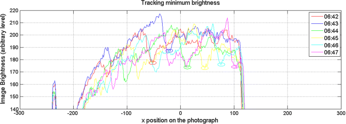

  

  Brightness of the photograph along the cross section shown by the red dotted line in Fig. 12 from 0642 LT to 0647 LT. The circles indicate the selected positions on the image used for calculating the phase velocity of the KH wave

The photographs also provided information about the spanwise extent of the KH billows. Table 1 and Fig. 14 indicate that the transverse dimension of the largest billows was less than twice the horizontal wavelength (typically 6000 m). Therefore, the large-amplitude KH billow patch covered a horizontal extent of ~ 24 km × 6 km only. This could indicate a localized KH instability event even if the stability conditions conducive to the generation of the KH billows might have been much more extended horizontally, according to the radar and radiosonde data.

Concluding remarks

The MU radar observed a train of deep KH billows inside a mid-level cloud, but close to the cloud base in an upper level front. Soon after their emergence in the radar image, they formed 3–4 smooth, coherent eddies and then collapsed. They were also detected by two lidars through their effects of ice particle entrainment by the KH billows.

• (1) The fish-eye camera captured the deformation of the cloud base produced by the vertical displacements due to KH billows about 1.0 km below the center of the billows. The photographs, collected every 1 min, confirmed the orientation of the phase front (~ 23° from north), horizontal wavelength (~ 3.7–4.0 km) and phase velocity (~ 17 ${\text{ms}}^{ - 1}$) deduced from wind and wind shear data.

• (2) In addition, the photographs indicated that the KH billows covered a horizontal domain that did not exceed 24 km streamwise and 6 km spanwise (i.e., less than twice their horizontal wavelength), indicating a very localized source. The complementary information provided by the photographs thus indicates that the time evolution revealed by the MU radar was dominated by the advection of billows at different stages of their evolution. They persisted over more than 8 min without noticeable deformation. Each billow forming the horizontal patch was likely not at the same stage of evolution: The first billows detected by the radar may have coincided with the earliest stage of the billows, at the edges of the patch, giving the appearance of growing KH billows in the radar images (see Fig. 2 between 06:45 and 07:00 LT). The radar did not show the real time evolution of the KH billow development (likely much slower than it can be deduced from the radar image if the apparent time evolution is interpreted as the time evolution of each KH structure). The radar observations are thus representative of their spatial distribution and do not provide information about their lifespan; the radar did not reveal the standard evolution of KH billows (i.e., wave amplification, breaking, mixing, possibly followed by the formation of a double-layer structure), but this evolution may have been confirmed if we were able to follow the KH billows in their motion with the background flow.

• (3) Strong turbulence (energy dissipation rates of the order of a few tens of ${\text{mWkg}}^{ - 1}$) occurred mainly near the edges of the billows, but also, to a lesser extent, in their core. It corresponds to moderate aviation turbulence.

• (4) The KH billow train observed inside the mid-level cloud but just above the cloud base was associated with a MCT layer immediately below the cloud base. In fact, the upper edge of the MCT was deeply indented due to the billows above. During another ShUREX campaign in 2016, we observed a very similar event under very similar conditions, with occurrence again of a train of high-amplitude KH billows just above a mid-level cloud base and a MCT layer underneath the cloud base. These were the only two instances during the three ShUREX campaigns (2015, 2016 and 2017) spanning over a total of 9 weeks, when we observed such spectacular, high-amplitude billows inside the mid-level cloud. In both cases, there was a MCT immediately below the cloud base. We do not know if the simultaneous presence of KH billows inside the cloud and MCT below the cloud base in these two instances is a mere happenstance. If it is not, then the dynamical mechanism responsible for simultaneous occurrence of shear instability above and convective instability below the cloud base needs to be explored. It is worth noting that MCT arises due to rapid sublimation in the dry air layer below the cloud base, of ice particles falling down from the cloud into the dry layer. These particles might have originated from condensation of ice nuclei inside the cloud immediately above the cloud base. Are the two events dynamically related? If so, how? We do not know the answer to these questions.

References

Behrendt A, Nakamura T, Tsuda T (2004) Combined temperature lidar for measurements in the troposphere, stratosphere, and mesosphere. Appl Opt 43(14):2930–2939
Blumen W, Banta RM, Burns S, Fritts DC, Newsom R, Poulos GS, Sun J (2001) Turbulence statistics of a Kelvin–Helmholtz billow event observed in the night-time boundary layer during the CAES-99 filed program. Dyn Atmos Oceans 34:189–204
Campbell JR, Hlavka DL, Welton EJ, Flynn CJ, Turner DD, Spinhirne JD, Scott VS, Hwang IH (2002) Full-time, eye-safe cloud and aerosol lidar observation at atmospheric radiation measurement program sites: instruments and data processing. J Atmos Ocean Technol 19:431–442
Durran DR, Klemp JB (1982) On the effects of moisture on the Brünt–Väisälä frequency. J Atmos Sci 39:2152–2158
Fritts DC, Palmer TL, Andreassen O, Lie I (1996) Evolution and breakdown of Kelvin–Helmholtz billows in stratified compressible flows. Part I: comparison of two- and three-dimensional flows. J Atmos Sci 53:3173–3191
Fukao S, Sato T, Tsuda T, Yamamoto M, Yamanaka MD (1990) MU radar—new capabilities and system calibrations. Radio Sci 25:477–485
Fukao S, Luce H, Mega T, Yamamoto MK (2011) Extensive studies of large-amplitude Kelvin–Helmholtz billows in the lower atmosphere with VHF middle and upper atmosphere radar. Q J R Meteorol Soc 137:1019–1041
Kantha L, Lawrence D, Luce H, Hashiguchi H, Tsuda T, Wilson R, Mixa T, Yabuki M (2017) Shigaraki UAV-radar experiment (ShUREX 2015): an overview of the campaign with some preliminary results. Prog Earth Planet Sci 4:19. https://doi.org/10.1186/s40645-017-0133-x
Kirshbaum DJ, Durran DR (2004) Factors governing cellular convection in orographic precipitation. J Atmos Sci 61:682–698
Klostermeyer J, Rüster R (1981) Further study of a jet stream-generated Kelvin–Helmholtz instability. J Geophys Res Atmos 86:6631–6637
Kudo A (2013) The generation of turbulence below midlevel cloud bases: the effect of cooling due to sublimation of snow. J Appl Meteorol Climatol 52(819–833):20153
Kudo A, Luce H, Hashiguchi H, Wilson R (2015) Convective instability underneath midlevel clouds: comparisons between numerical simulations and VHF radar observations. J Appl Meteorol Climatol 54:2217–2227
Long CN, Sabburg JM, Calbó J, Pagès D (2006) Retrieving cloud characteristics from ground-based daytime color all-sky images. J Atmos Ocean Technol 23:633–652
Luce H, Yamamoto M, Fukao S, Hélal D, Crochet M (2001) A frequency radar interferometric imaging applied with high resolution methods. J Atmos Sol Terr Phys 63:221–234
Luce H, Hassenpflug G, Yamamoto M, Fukao S, Sato K (2008) High resolution observations with MU radar of a KH instability triggered by an inertia-gravity wave in the upper part of a jet-stream. J Atmos Sci 65:1711–1718
Luce H, Mega T, Yamamoto MK, Yamamoto M, Hashiguchi H, Fukao S, Nishi N, Tajiri T, Nakazato M (2010) Observations of Kelvin–Helmholtz instability at a cloud base with the MU and weather radars. J Geophys Res Atmos 115:D19116. https://doi.org/10.1029/2009JD013519
Palmer RD, Yu T-Y, Chilson PB (1999) Range imaging using frequency diversity. Radio Sci 34:1485–1496
Sassen KWP, Patrick Arnott W, O’Starr DO, Mace GG, Wang Z, Poellot MR (2003) Midlatitude cirrus clouds derived from Hurricane Nora: a case study with implications for ice crystal nucleation and shape. J Atmos Sci 60:873–891
Schultz DM et al (2006) The mysteries of mammatus clouds: observations and formation mechanisms. J Atmos Sci 63:2409–2435
Spinhirne JD (1993) Micro pulse lidar. IEEE Trans Geosci Remote Sens 31:48–55
Thorpe SA (1973) Experiments on instability and turbulence in stratified shear flow. J Fluid Mech 61:731–751
White AB, Lataitis RJ, Lawrence RS (1999) Space and time filtering of remotely sensed velocity turbulence. J Atmos Ocean Technol 16:1967–1972
Wilson R, Luce H, Hashiguchi H, Nishi N, Yabuki M (2014) Energetics of persistent turbulent layers underneath mid-level clouds estimated from concurrent radar and radiosonde data. J Atmos Sol Terr Phys 118:78–89
Authors’ contributions
HL performed the radar, balloon and fish-eye camera data processing with assistance from HH and LK. MY performed the lidar data processing. HH, MY and LK participated in the synthesis of the study results. All authors read and approved the final manuscript.
Acknowledgements
This study was supported by JSPS KAKENHI Grant Number JP15K13568 and the research Grant for Mission Research on Sustainable Humanosphere from Research Institute for Sustainable Humanosphere (RISH), Kyoto University. The MU radar belongs to and is operated by RISH. We express our sincere thanks to Dr. Shiobara at National Institute of Polar Research for providing MPL system.
Competing interests
The authors declare that they have no competing interests.
Availability of data and materials
Data are not yet available because they are still being analyzed for follow-on studies and papers.
Funding
This study was supported by JSPS KAKENHI Grant Number JP15K13568 and the research grant for Mission Research on Sustainable Humanosphere from Research Institute for Sustainable Humanosphere (RISH), Kyoto University. The MU radar belongs to and is operated by RISH, Kyoto University.
Publisher’s Note
Springer Nature remains neutral with regard to jurisdictional claims in published maps and institutional affiliations.
Author information
Authors and Affiliations
Corresponding author
Rights and permissions
Open Access This article is distributed under the terms of the Creative Commons Attribution 4.0 International License (http://creativecommons.org/licenses/by/4.0/), which permits unrestricted use, distribution, and reproduction in any medium, provided you give appropriate credit to the original author(s) and the source, provide a link to the Creative Commons license, and indicate if changes were made.
About this article
Cite this article
Luce, H., Kantha, L., Yabuki, M. et al. Atmospheric Kelvin–Helmholtz billows captured by the MU radar, lidars and a fish-eye camera. Earth Planets Space 70, 162 (2018). https://doi.org/10.1186/s40623-018-0935-0
Received:
Accepted:
Published:
DOI: https://doi.org/10.1186/s40623-018-0935-0