- Letter
- Open access
- Published:
The cause of heavy damage concentration in downtown Mashiki inferred from observed data and field survey of the 2016 Kumamoto earthquake
Earth, Planets and Space volume 69, Article number: 3 (2017)
Abstract
To understand the cause of heavy structural damage during the mainshock (on April 16, 2016) of the 2016 Kumamoto earthquake sequence, we carried out a field survey from April 29 through May 1, 2016, in Mashiki where heavy damage concentration was observed. The heavy damage concentration in downtown Mashiki could be understood based on the observed strong motions with the Japan Meteorological Agency instrumental seismic intensity of VII and information collected by the field investigation. First, the fundamental features of the structural damage in downtown Mashiki were summarized. Then, a distribution map of peak frequencies was derived from horizontal-to-vertical spectral ratios of microtremors. We could not see any systematic correlation between the peak frequencies and spatial distribution of damage ratios. We also analyzed observed strong motion data at two sites to obtain fling-step-like motions in the displacement time histories through the double integration of unfiltered accelerograms. It turned out that at both strong motion observation sites in Mashiki, only the east–west (EW) components had very strong velocity pulses westward before the emergence of the fling-step-like motion eastward, which would be the primary cause of heavy structural damage in downtown Mashiki, not site effects nor the fling-step-like motion itself.
Background
The 2016 Kumamoto earthquake sequence, which included a foreshock with MJMA of 6.4 on April 14, 2016, and a mainshock with MJMA of 7.3 on April 16, 2016, created heavy structural damage in several areas in Kumamoto Prefecture, Japan. The major rupture of the foreshock was considered to have emerged on the northernmost segment of the Hinagu fault, while that of the mainshock was primarily associated with the predefined Futagawa fault with some extension to the east, into the Aso caldera (GSI 2016). The heavily damaged areas of wooden houses spread in a narrow belt (~50 km long) alongside these two faults, from the southeast of Kumamoto City to the northwest of Minami-Aso Village. The notable exception was the damage concentrated area (DCA) in downtown Mashiki, where more than 80% of heavy damage ratios on wooden houses had been reported in several 100-m survey grids (JANDR 2016), even though the area is located about 3 km north of the main Futagawa fault.
It is quite fortunate for researchers that there are two permanent stations for strong motion observations in Mashiki. One is the KiK-net station KMMH16 (Okada et al. 2004) on the northeastern boundary of the DCA, and the other is the Kumamoto Prefecture’s Instrumental Intensity Seismometer (hereafter IIS) on the first floor of the Mashiki Town Hall building (a reinforced concrete building with three floors), which is located at the edge of the DCA. They observed both the foreshock and mainshock motions, whose JMA instrumental intensities (Karim and Yamazaki 2002) were reported to be VII, the highest intensity corresponding to the Modified Mercalli Intensity (MMI) of X to XII. Please note that there is no simple way to translate JMA instrumental intensities into MMI because MMI is the actual phenomenological index while JMA intensities do not directly correlate with phenomena associated with the ground shaking. The acceleration response spectra at the Kumamoto Prefecture’s IIS were quite large, larger than the observed ground motions at JR Takatori during the 1995 Kobe earthquake (e.g., Sakai 2016).
Thus, it is clear that the heavy damage in downtown Mashiki was caused by the strong ground motions in the area. However, which part of the strong motions contributed most to the heavy damage concentration during the mainshock, and how strong motion characteristics were generated, would be indispensable questions to answer for future mitigation of structural damage from similar crustal earthquakes.
To that end we carried out a field survey from April 29 through May 1, 2016, on structural damage in Mashiki and performed single-station microtremor observations with about 100-m grid points. In this paper, first, we report the important features of structural damage in the DCA and the spatial distribution of fundamental peak frequencies of the horizontal-to-vertical spectral ratios of the microtremors (MHVRs). We then report on the damage potential of the observed records at two sites by using the theoretical model for prediction of damage to wooden houses based on statistics from the Hyogo-ken Nanbu earthquake of 1995 (Nagato and Kawase 2000; Yoshida et al. 2005). Finally, we look for the emergence of the fling-step-like motions in the displacement seismograms and extract their contributions from the velocity seismograms to assess their effects on the damage potential.
Damage survey
First, the fundamental features of the structural damage in the DCA in downtown Mashiki were extracted and summarized. Figure 1 shows the schematic view of the DCA in downtown Mashiki. The damage concentration starts from the west of the national road route 443, running in the north–south (NS) direction, and extends until east of the prefectural road route 235, about 1.5–2 km in the east–west (EW) direction. In the NS direction, the width of the DCA is smaller, about ±300 m on average, spreading over the both sides of the prefectural road route 28, but the width increases as we move to the east and suddenly disappears from the national road route 443 even further east. The main features necessary to report the damage inside the DCA are as follows.

A schematic view of the damage concentrated area (DCA) in downtown Mashiki; Stars indicate the location of the two strong motion observation sites and circles represent the approximate locations of damaged buildings in the Figures
-
1.
Inside the DCA, not only old and weak wooden houses but also new and reinforced houses were damaged, although the percentage of the latter is smaller (Fig. 2).
Fig. 2 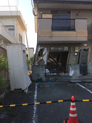
An example of a damaged apartment in the northern part of the DCA, which was constructed after the code modification in 1981
-
2.
The damaged houses look aligned to some lateral extent (about 50 to 100 m) in the EW direction.
-
3.
Many old houses successfully survived outside of the heavy damage lines in the EW direction, even inside the DCA (Fig. 3).
Fig. 3 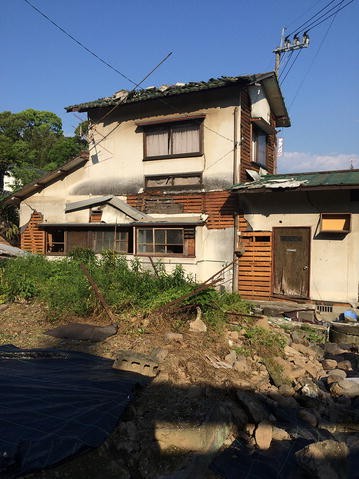
An example of an old house that scarcely survived in the eastern part of the DCA
-
4.
The deformed direction of the collapsed or heavily inclined houses was mostly in the EW direction. The overturning direction of tombstones and retaining walls for artificially filled soil were also mostly in the EW direction (Figs. 4, 5, 6).
Fig. 4 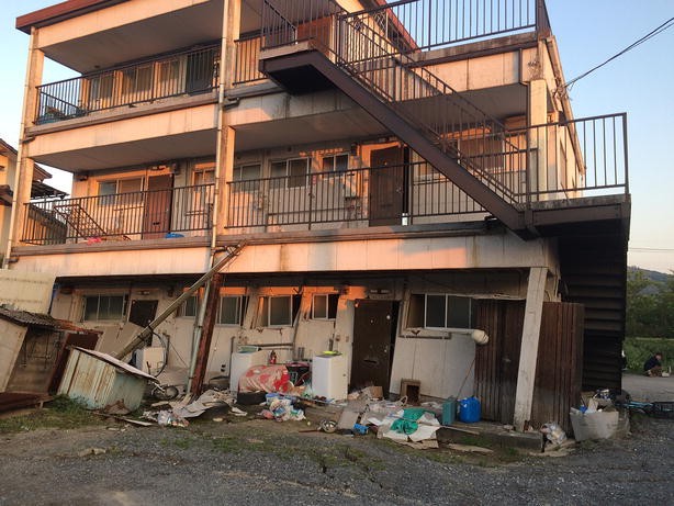
An example of a heavily inclined house predominantly in the EW direction
Fig. 5 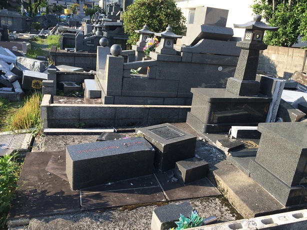
Overturning direction of tombstones was also in the EW direction
Fig. 6 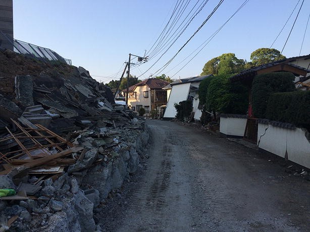
Direction of retaining wall failures for reclaimed land was also in the EW direction
-
5.
Significant ground deformation, failure, and cracks can almost always be seen on the paved roads crossing the above damage lines.


From these observations, one can see the possibility of the strong contribution of fling-step-like motions associated with the slip on the seismogenic fault. As was observed in Kobe during the 1995 Hyogo-ken Nanbu earthquake, the asperity pulse generated by the directivity in the fault-normal component (Matsushima and Kawase 1999) was not a primary cause of the DCA in downtown Mashiki, since the strike of the Futagawa fault is about N60°E, closer to the EW direction. We also needed to obtain a predominant frequency distribution of the ground in order to evaluate the possibility of strong site effects as the cause of the DCA, such as the basin-edge effect that was the case of the damage belt in Kobe during the 1995 Hyogo-ken Nanbu earthquake (Kawase 1996; Matsushima and Kawase 1999).
Microtremor observations
To explain the shape of the DCA, we needed to investigate the effects of the local basin structure from the surface down to the bedrock. We are currently working on the S-wave velocity inversion (Nagashima et al. 2014) based on the horizontal-to-vertical spectral ratios of earthquake (EHVRs) motions in and around the DCA through the theory of diffuse fields (Kawase et al. 2011), which will be reported separately. Here we would like to report our preliminary result on the predominant frequency distribution obtained from MHVRs with every 50- to 100-m grid covering most of the DCA. Measurements were taken for 15 to 20 min at one location. Before calculating the Fourier spectra of observed three component accelerograms, we selected stable parts without strong yet transient noise contributions. The data processing was performed following the standardized procedure (e.g., Mori et al., 2016), in which 40.96-s record sections were extracted with 50% overlapping, and Fourier spectra were then obtained with the 0.1 Hz Parzen window for smoothing, and finally, all available spectral ratios of the MHVRs from Fourier spectra were stacked and averaged.
In Fig. 7, we plot the locations of the measured microtremor sites, in total 71 locations, together with the locations of two strong motion sites. The site numbers are shown at representative sites. Figure 8 shows the distribution of the fundamental peak frequency of MHVRs at every location observed. A larger size balloon indicates a higher peak frequency, the value of which is shown in the center of each balloon. We cannot see much correlation of heavy damage to the predominant frequency. Since the predominant frequency ranges from 1 to 4 Hz, the thickness of the sediments in the DCA should vary from one to four times (or the average velocity should vary from one to four times). Such a large difference in the soil properties should be reflected in the soil amplification and therefore in the damage distribution. Because there is no apparent correlation of the predominant frequency distribution with the damage distribution, we may conclude that the damage concentration is not primarily controlled by spatial differences in the local site effects, specifically featured in the DCA. Note that the peak frequency in MHVRs at two strong motion stations were quite close to the peak frequency in EHVRs there, as is the case at 100 sites in Japan (Mori et al. 2016). For the cause of a 3-Hz peak frequency at KMMH16, by either MHVR or EHVR, we can refer to the velocity structure obtained there by PS logging in a 200-m borehole (NIED 2016).

Locations of the measured microtremor sites and two strong motion observation sites; the site numbers are shown at representative sites, and the same DCA boundary from Fig. 1 is also shown

Fundamental peak frequency of MHVRs at 71 locations observed in downtown Mashiki; the size of the circle at each site corresponds to its peak frequency; the same DCA boundary from Fig. 1 is also shown
There are a couple of preliminary reports that suggest the strong contribution of the local site amplification in the DCA. For example, Nagao (2016) found a strong correlation of damage distribution with site amplification characteristics. The reason for his statement is primarily that the damaged wooden houses were found to be concentrated in the region south of the prefectural road route 28. Actually, this is not the case, since we have also found numbers of heavily damaged or collapsed houses to the north of the route 28, as shown in Fig. 1. In the northern part of the DCA, we cannot see any significant spatial differences in the predominant frequencies in MHVRs, as shown in Fig. 8.
Damage evaluation by the prediction model
Since there were so many heavily damaged or toppled wooden houses in the DCA, we needed to first use the constructed theoretical model to reproduce the heavy damage distribution in Kobe during the 1995 Hyogo-ken Nanbu earthquake (Nagato and Kawase 2000; Yoshida et al. 2005). The merit of using this theoretical model, together with the observed strong accelerograms, is that the effects of ground motion characteristics to the structural damage could be investigated through the predicted damage ratios from the model.
In Fig. 9, we plot accelerograms of the mainshock at two strong motion sites, namely KiK-net KMMH16 and IIS Mashiki Town Hall. The timing of the initial arrivals was aligned by sight. We can see that the waveforms at both sites share quite common features, since the separation between them is about 700 m, but that waveforms at KMMH16 have more high-frequency power than those at IIS Mashiki Town Hall. In Table 1, we summarize the predicted damage ratios based on the theoretical models for wooden structures with different average capacities based on their construction ages (Yoshida et al. 2005). For houses built after 1982, the predicted damage ratios are only 10–15%, while for those built before 1982 they are 30–70%, increasing with construction age. We should note that the EW components at both sites show stronger power of damage potential than the NS components, which may come from the clear 1-s pulse at 20 to 21 s in Fig. 9. We also need to mention that records at KMMH16 have stronger power for younger houses (with high natural frequencies) while those at IIS Mashiki Town Hall have stronger power for older houses (with lower natural frequencies). This is because the records at KMMH16 are richer in high-frequency components than those at IIS Mashiki Town Hall, while the latter is richer in low-frequency components.

Accelerograms of the mainshock at two strong motion sites, KiK-net KMMH16 and IIS Mashiki Town Hall
Fling-step extraction
Because of the clear surface displacement inferred from Interferometric Synthetic Aperture Rader (InSAR) along the Futagawa–Hinagu fault system (GSI 2016; JANDR 2016), there is no doubt that the observed ground motions in downtown Mashiki were contributed by the fling-step motion caused by the surface emergence of the fault rupture. At first we thought that the fling-step would be a primary source of the DCA in Mashiki. Therefore, we integrated the observed accelerograms twice to get displacement seismograms at two stations in Mashiki and tried to extract the fling-step-like motions from the velocity seismograms to see the effects in terms of the damage potential.
Figure 10 shows the displacement seismograms at KMMH16 and IIS Mashiki Town Hall. We can see quite similar permanent offsets at these two sites in all three components, which is quite natural considering the distance between them. The permanent offsets in three directions are quite consistent with those inferred from InSAR at downtown Mashiki (GSI 2016; JANDR 2016).

Displacement seismograms at KMMH16 and IIS Mashiki Town Hall as calculated by double integrations from accelerograms without any filtering; black broken lines indicate the estimated ramp functions to extract the fling-step like motions, while the gray dotted lines on the two horizontal component graphs are the values in the perpendicular direction, for comparison
To simulate fling-step-like motions in these seismograms, we used a simple sine ramp function (one sine pulse in acceleration) and determined three appropriate parameters: the starting time, rise time, and final offset. The final functions are shown by black broken lines in Fig. 10.
As is evident, such a simple function can explain quite well the fling-step-like motions in these seismograms. We should note, however, that the starting time in the EW component was about 1 s delayed in comparison with those in the NS and up–down (UD) components. Because of this delay, the velocity pulse prominent in the EW component at 20–21 s would not be affected at all by the fling-step-like contribution, as shown in Fig. 11. Conversely, the velocity pulse in the NS component was reduced by 1/3 if we extract the fling-step contribution.

Velocity seismograms at KMMH16 and IIS Mashiki Town Hall calculated by one time integration from accelerograms without any filtering; black broken lines indicate velocity contributions of the estimated ramp functions shown in Fig. 10
We should note that the time shift of the fling-step-like motions can be observed in Fig. 10. It may not be totally appropriate to call the determined smoothed rump functions as fling-step functions, but what we determined here was the best matching smooth function for the observed displacement time history of each component. Because the observed displacement time history in the EW direction at both IIS Mashiki and KiK-net KMMH16 have about 1-s delayed start-up and stopping timings in comparison with the NS and UD components (with almost the same rise time), the timing in the velocity functions in Fig. 11 is also delayed. The time delay would not be affected by the functional form used to represent the fling-step-like motions.
As a matter of course, we can obtain the same start-up and stopping timing for all three components, if we optimize the matching to observed components with a single function. However, if we do so, the degree of matching to that common function would be less, since the start-up and stopping timings in the EW component were delayed about 1 s, as we see in the differences between the black broken lines and gray dotted lines in Fig. 10. The purpose of the investigation here into the functional characteristics of fling-step-like motions was to see their contributions to the velocity seismograms in Fig. 11 and hence identify the cause of the DCA in Mashiki. We do not intend to extract the real functional form of the fling-step motions generated as the direct consequence of the rupture on the fault.
The geophysical interpretation of the observed fling-step-like motions should be investigated further, but it is not the subject of this paper. We would like to refer to the study of Bouchon et al. (2002) for the Izumit, Turkey, earthquake of 1999 on the velocity ground motions observed at the site near the rupture initiation point, IZT. We can see the initial pulse to the opposite direction of the fault motion as seen here in Mashiki, although the amplitude of that pulse was much less.
Discussion
The presented materials showed that the primary source of the DCA in Mashiki would be a strong velocity pulse in the EW component, reaching the level of 150–160 cm/s. The source of such a strong velocity pulse, however, is not yet clear at this stage of investigation. From delineated predominant frequencies in the area, it is not likely to be caused by strong local site effects as was the case in Kobe, although a certain amount of amplification may contribute to increases in the peak ground velocity. When we look at the evidence of the fling-step contribution, we successfully reproduced observed fling-step-like motions by using a simple smoothed ramp function. However, the contribution did not reduce the peak ground velocity in the EW component at all, because the peak-out timing of the fling-step-like motions was not coincident with that of the maximum velocity pulse in the EW component.
This means that we need to have a significant contribution of energy from the source before the arrival of the major fling-step-like motion at Mashiki. What could be a possible source of the observed velocity pulse predominantly in the fault-parallel component? Promising evidence is provided from the strong motion simulation study by Bouchon et al. (2002) for the 1999 Izumit, Turkey, earthquake, as mentioned above. Since the amplitude of the initial pulse in the opposite direction to the fault motion is much less than the observed one in Mashiki, we need to investigate the possible configuration of the source near the hypocenter.
On the other hand, Miyatake (2000) has suggested one rupture scenario of a vertical strike-slip fault with a strong directivity effect in the fault-parallel component, that is, vertical rupture propagation on a source located immediately below the observation site. If we can have some marginal amount of slip on the segment below downtown Mashiki near the rupture initiation point, we may see a velocity pulse due to the directivity in the fault-parallel component as seen in Miyatake (2000). The problem with this hypothesis is that the produced fault-parallel motion from such a scenario would be moving in the positive direction of the fault motion, opposite to the observed pulse. This means that downtown Mashiki should be located to the south of the asperity that generates this directivity pulse. We are now looking for arrival of the same pulse at stations around downtown Mashiki.
Conclusions
Through a damage survey in downtown Mashiki and subsequent simulation using the theoretical damage prediction model, dense microtremor array measurements for a predominant frequency distribution map, and the extraction of the fling-step components from the velocity seismograms, we found that the observed damage dominated in the EW direction could be due to a velocity pulse close to the fault-parallel component and that the fling-step contribution could not be a primary source of that strong velocity pulse. Since there was no strong correlation of peak frequency distribution with the damage concentration in Mashiki, we believe that the strong velocity pulse was generated primarily by a simple source process adjacent to the rupture initiation point. We need to invert a detailed rupture process, specifically focused on the fault-parallel component in Mashiki and other adjacent areas, where we can see similar velocity pulses in the observed seismograms.
Abbreviations
- DCA:
-
damage concentrated areas
- EHVRs:
-
earthquake horizontal-to-vertical spectral ratios
- EW:
-
east–west
- IIS:
-
instrumental intensity seismometer
- InSAR:
-
interferometric synthetic aperture rader
- JMA:
-
Japan Meteorological Agency
- MHVRs:
-
microtremor horizontal-to-vertical spectral ratios
- MMI:
-
modified mercalli intensity
- NS:
-
north–south
- UD:
-
up–down
References
GSI GeoSpatial Information Authority, Japan (2016) The 2016 Kumamoto earthquake: crustal deformation around the faults. http://www.gsi.go.jp/ BOUSAI/H27-kumamoto-earthquake-index.html. Accessed 30 July 2016 (in Japanese)
Bouchon M, Toksöz MN, Karabulut H, Bouin M-P, Dietrich M, Aktar M, Edie M (2002) Space and time evolution of rupture and faulting during the 1999 İzmit (Turkey) earthquake. Bull Seism Soc Am. 92:256–266. doi:10.1785/0120000845
JANDR, Japan Academic Network for Disaster Reduction (2016) Kumamoto Earthquake; three months after. http://janet-dr.com/11_saigaiji/160716kyushu_houkokukai/ 20160716pdf/00_160716_all.pdf. Accessed 30 July 2016 (in Japanese)
Karim KR, Yamazaki F (2002) Correlation of JMA instrumental seismic intensity with strong motion parameters. Earthq Eng Struct Dyn 31:1191–1212. doi:10.1002/eqe.158
Kawase H (1996) The cause of the damage belt in Kobe: “The Basin-Edge Effect”, constructive interference of the direct S-wave with the basin-induced diffracted/Rayleigh Waves. Seism Res Lett 67:25–34
Kawase H, Sánchez-Sesma FJ, Matsushima S (2011) The optimal use of horizontal-to-vertical (H/V) spectral ratios of earthquake motions for velocity structure inversions based on diffuse field theory for plane waves. Bull Seism Soc Am 101:2001–2014. doi:10.1785/0120100263
Matsushima, S and H Kawase (1999) 3-D wave propagation analysis in Kobe referring to ‘The basin-edge effect, in Effect of Surface Geology on Strong Motions, Vol. 3, eds. Irikura et al. (Balkema, Rotterdam). 1377–1384
Miyatake T (2000) Computer simulation of strong ground motion near a fault using dynamic fault rupture modeling: spatial distribution of the peak ground velocity vectors. Pure Appl Geophys 157: 2063–2081
Mori Y, Kawase H, Matsushima S, Nagashima F (2016) Comparison of observed earthquake and microtremor horizontal-to-vertical spectral ratios and inversion of velocity structures based on their empirical ratios. J JAEE 16(9):13–32 (in Japanese with English abstract)
Nagao, T. (2016) Survey results and remaining issues of the Kumamoto earthquake, http://www2.kobe-u.ac.jp/~nagaotak/kumamotover10.pdf Accessed 10 Nov 2016
Nagashima F, Matsushima S, Kawase H, Sánchez-Sesma FJ, Hayakawa T, Satoh T, Oshima M (2014) Application of horizontal-to-vertical (H/V) spectral ratios of earthquake ground motions to identify subsurface structures at and around the K-NET site in Tohoku, Japan. Bull Seism Soc Am 104(5):2288–2302. doi:10.1785/0120130219
Nagato K, Kawase H (2000) A set of wooden house models for damage evaluation based on observed damage statistics and non-linear response analysis and its application to strong motions of recent earthquake. In: Proceedings of the 11th Japan Earth Eng Symp
NIED National Research Institute for Earth Science and Disaster Resilience (2016) A strong-motion seismograph networks Portal site. http://www.kyoshin.bosai.go.jp/ Accessed 30 July 2016
Okada Y, Kasahara K, Hori S, Obara K, Sekiguchi S, Fujiwara H, Yamamoto A (2004) Recent progress of seismic observation networks in Japan -Hi-net, F-net, K-NET and KiK-net-. Earth Planets and Space 56:15–18
Sakai, Y (2016) Comparison with the ground motions in the Kumamoto Earthquake (4/16 01:25) and past intensive ground motions. http://www.kz.tsukuba.ac.jp/~sakai/kmm_hk2_en.htm. Accessed 30 July 2016
Yoshida K, Hisada Y, Kawase H, Fushimi M (2005) Construction of vulnerability function of Japanese wooden houses for the best index of the destructive potential. In: AIJ Annual Meeting Proceedings, B-2, 161-162 (in Japanese)
Authors’ contributions
HK, SM, FN, and KN performed field investigations. HK and B contributed to the structural damage simulation. HK, SM, and FN participated in microtremor analysis. HK wrote the initial draft of the manuscript through discussion with SM, FN, B, and KN. All authors read and approved the final manuscript.
Acknowledgements
This work was partly supported with the Grant-in-Aid for Special Purposes (16H06298: P.I. Hiroshi Shimizu), the Grant-in-Aid for Basic Research A (26242034: P.I. Hiroshi Kawase), and the DPRI internal fund for the Kumamoto earthquake emergency investigation activities. We thank the students of Kawase and Matsushima Laboratories of DPRI who supported the field investigation in the target area. Thanks are extended to NIED for KiK-net strong motion data and JMA for IIS data through collaboration with the Kumamoto Prefectural Government. In Figs. 1 through 3, road map and satellite images from Google maps (https://www.google.co.jp/maps) were used.
Competing interests
The authors declare that they have no competing interests.
Author information
Authors and Affiliations
Corresponding author
Rights and permissions
Open Access This article is distributed under the terms of the Creative Commons Attribution 4.0 International License (http://creativecommons.org/licenses/by/4.0/), which permits unrestricted use, distribution, and reproduction in any medium, provided you give appropriate credit to the original author(s) and the source, provide a link to the Creative Commons license, and indicate if changes were made.
About this article

Cite this article
Kawase, H., Matsushima, S., Nagashima, F. et al. The cause of heavy damage concentration in downtown Mashiki inferred from observed data and field survey of the 2016 Kumamoto earthquake. Earth Planets Space 69, 3 (2017). https://doi.org/10.1186/s40623-016-0591-1
Received:
Accepted:
Published:
DOI: https://doi.org/10.1186/s40623-016-0591-1