A new global empirical model of the electron temperature with the inclusion of the solar activity variations for IRI

Abstract

A data-base of electron temperature (T_e) comprising of most of the available LEO satellite measurements in the altitude range from 350 to 2000 km has been used for the development of a new global empirical model of T_e for the International Reference Ionosphere (IRI). For the first time this will include variations with solar activity. Variations at five fixed altitude ranges centered at 350, 550, 850, 1400, and 2000 km and three seasons (summer, winter, and equinox) were represented by a system of associated Legendre polynomials (up to the 8th order) in terms of magnetic local time and the earlier introduced invdip latitude. The solar activity variations of T_e are represented by a correction term of the T_e global pattern and it has been derived from the empirical latitudinal profiles of T_e for day and night (Truhlik et al., 2009a). Comparisons of the new T_e model with data and with the IRI 2007 T_e model show that the new model agrees well with the data generally within standard deviation limits and that the model performs better than the current IRI T_e model.

1. Introduction

There were numerous attempts to empirically describe and model solar activity variations of the electron temperature in the upper ionosphere and plasmasphere e.g. Evans (1973), Mahajan and Pandey (1979), Bilitza and Hoegy (1990), Truhlik et al. (2001), Webb and Essex (2003), and Sharma et al. (2010) but so far no model describes this feature accurately and it is therefore not yet included in the IRI model. The elementary mechanisms that play an important role in the T_e variation with solar flux seem to be broadly understood. The electron temperature is determined by the balance of heating through photoelectrons that are created by the solar EUV irradiance, cooling through collisions with neutrals and ions, and heat conduction along magnetic field lines. All three terms increase with solar activity due to the increase in EUV flux, neutral density, neutral temperature, and electron and ion densities. Since these processes compensate each other, the result could be a T_e increase, decrease, or no change at all (e.g. Bilitza et al, 2007 and references therein). So while almost all ionospheric parameters increase with solar activity electron temperature is the one parameter that shows a more complex solar activity dependence. There are two main reasons why modeling of the solar activity variations of the electron temperature is a very difficult task:

• (a) Changes of T_e caused by solar activity variations are comparable or even below the day-to-day variability and scatter of T_e values, which is particularly important in daytime. Thus, the solar activity variation of T_e is often hidden in the data scatter.

• (b) Frequent inconsistency among various T_e data sets especially in regimes of low electron density because most techniques for measuring T_e depend critically on the presence of a sufficient number of electrons.

Truhlik et al. (2009a) using a large data-base comprising of almost all available satellite data established latitudinal empirical profiles of the electron temperature for three levels of solar activity (high, medium and low), three seasons (summer, winter and equinox), five altitude ranges (350, 550, 850, 1400, and 2000 km) and two local times (day and night). In this paper we use the results from Truhlik et al. (2009a) and we incorporate them into a new global empirical model of the electron temperature. The following sections describe this model in detail.

2. Data

Our data-base which stretches over four solar cycles has been described in detail in Bilitza et al. (2007). It includes data from the early Explorers (31) up to the ongoing DMSP satellites. The altitude distribution of data is shown in Fig. 1.

Fig. 1.

Distribution of data versus altitude from all data sets include in our data base.

Bilitza et al. (2007) pointed out that in combining T_e data from different satellites it is extremely important to assess the data quality of the individual data sets and to discard or correct data sets with known contamination problems. We follow their conclusions and besides their changes made to individual data sets, we have made several additional changes. All changes that we use for the new model we summarize as follows (see also Truhlik et al., 2009a, b):

• (1) ISIS-1 data were included only above 1500 km and were reduced by 15%. The altitude threshold was introduced because the ISIS-1 data at lower altitudes show discrepancies with several of the other data sets. The reduction factor at high altitudes is a compromise based on the arguments given by Köhnlein (1986) and by Webb and Essex (2003) and also on our own comparisons with data from Intercosmos 24 and 25.

• (2) Explorer 31 data were now included but only above 1500 km altitude because the T_e probe of this mission is of a similar construction as the T_e probe onboard ISIS-1 and the measured T_e values indicated similar concerns as for ISIS-1 data.

• (3) From Intercosmos 19 only data from altitudes above 750 km were included because the probe produces unrealistically high T_e for N_e > 5 · 10¹¹ m⁻³.

• (4) In the case of Intercosmos 24 and 25 the temperature was determined as the median of T_ex, T_ey, and T_ez (identical instruments on both satellites consisted of three T_e planar sensors in directions x, y and z; see Truhlik et al. (2001) for more detail).

• (5) From the DMSP T_e measurements only data for solar activity PF_10.7 > 120 (for PF_10.7 definition see next section) were taken because the low solar activity (= low density) temperature data are unrealistically high (see Bilitza et al., 2007). Also, we have selected only those data with “quality flag” 1 or 2 as recommended by DMSP SSIES team on http://cindispace.utdallas.edu/DMSP/.

• (6) As a new data set we have added the temperature measurements of the Indian SROSS C2 satellite.

Some of the data sets have very high time resolution, much higher than required for our modeling purposes. In these cases we have averaged the data to a 100 second time resolution. The total number of measurements in our database is about 9 million data points across 20 satellites.

3. Model Formulation

Based on the altitude distribution of data in our database (see Fig. 1) and on the need to cover all important height regimes, we have selected the following anchor altitudes for our model: 350, 550, 850, 1400 and 2000 km. Similar to Brace and Theis (1981) and Truhlik et al. (2000) we have averaged data on a local time-latitude grid and modeled global variations using a spherical harmonics expansion to 8th order. In the first step, we have built the core T_e model using the T_e average in each bin. In the second step, we have created a term describing the solar activity variations in the bins based on the earlier work by Truhlik et al. (2009a). The solar activity variation term is used as an additive term to the core model. After the global models are established for the 5 fixed altitudes they are combined to produce the full altitude profile in the same way as it is done now in the IRI model. The IRI approach is based on the Booker-Epstein formalism (e.g. Bilitza, 1990) which divides the profile into regions of constant gradient with the boundaries given by the 5 fixed altitudes. Epstein-step functions are used to transition from one region to the next thus generating a continuous analytical representation of the T_e gradient and integration then results in the final T_e formula. For future upgrades of the IRI model physics-based field aligned profile functions as for example deduced by Bilitza (1975), Titheridge (1998), or Truhlik et al. (2009b) could bring further improvement.

3.1 The core model

The core model consists of submodels for individual altitude ranges and seasons. All available data were grouped by season (90 day periods centered on equinoxes and solstices) and for the following altitude ranges (similar to Truhlik et al., 2000): 350 ± 40 km, 550 ± 50 km, 850 ± 90 km, 1400 ± 150 km, and 2000 ± 300 km. For equinox we have combined data from spring and autumn (90 day periods centered on March 21 and September 23) from both hemispheres, because we consider possible hemispheric asymmetries as an influence of the 3rd order (1st order effects are related to local time, and altitude; 2nd order to season, and solar activity; 3rd order to longitude, and hemispheric differences). For solstices we have also combined data from both hemispheres (northern three months periods centered on June 21 and southern three months periods centered on December 21 for summer, and vice versa for winter). Magnetic local time (MLT) and latitude were chosen as the main coordinates. Longitudinal variation can be reduced to a second order effect if a latitudinal coordinate is chosen that takes into account the real configuration of the geomagnetic field. The latitudinal coordinate (invdip), introduced by Truhlik et al. (2001), is such a coordinate and it is used for our model. Invdip is defined as

(1)

where α = sin³ ǀ diplat ǀ and β = cos³(invl). Thus, invdip is close to the dip latitude (diplat) near the equator and gets closer to the invariant latitude (invl) at higher latitudes.

For each individual data group (height range and season) a system of associated Legendre polynomials up to the 8th order was employed as an expansion function

(2)

where

• = associated Legendre function

• θ = invdip colatitude (0 … π)

• φ = magnetic local time (0 … 2π).

Before applying this fitting procedure, medians of the common logarithm of T_e data were calculated on a invdip vs. MLT regular grid. The minimum number of bins in the grid was 9 vs. 18 to guarantee coefficients fully recoverable and free of aliasing effects (Martinec, 1991). Thus the bins width of this grid corresponds to the maximal order of Legendre polynomials (8th order) in Eq. (2). Medians of PF_10.7 pertaining to the T_e data (for each altitude and season) denoted as PF_10.7M were determined in each bin and they were used to calculate the solar activity term (see the next subsection).

3.2 The solar activity term

The solar index used for our model is the PF_10.7 index that is defined as PF_10.7 = (F_{10.7 A} + F_{10.7 d})/2 with F_{10.7 d} the daily F_10.7 solar radio flux index and F_{10.7 A} its 81-day average (3 solar rotations). PF_10.7 has been shown to have higher correlation with T_e than some of the other solar indices (e.g. Richards et al., 1994). In the first step to obtain the solar activity term we have developed a solar activity function denoted as fT_ePF_10.7 again for each altitude and season. This function describes how T_e depends on PF_10.7 as function of local time and latitude. But because of the limited amount of data available in each bin we had to reduce the number of MLT intervals to just two, a day (centered at 13 h MLT ± 2.5 h) and a night (centered at 1 h MLT ± 3 h) interval. Thus, we have obtained fT_ePF_{10.7 day} and fT_ePF_{410.7 night} in the first step. To construct this function we have adopted the latitudinal profiles from Truhlik et al. (2009a) that were derived for three levels of solar activity (high, medium and low) and day and night. The three levels of solar activity were defined in Truhlik et al. (2009a) as follows: (i) low PF_10.7 < 110; (ii) medium 110 ≤ PF_10.7 ≤ 180; (iii) high PF_10.7 > 180. We have taken the low solar activity level as the reference point and normalized the other two levels by determining the difference to this reference level (Figs. 2(a) and (b)). The normalized values were denoted as 0, ΔT_eml, and ΔT_ehl and corresponding values of solar activity PF_{10.7 l}, PF_{10.7 m}, and PF_{10.7 h} were determined as medians in each latitude bin for the three intervals (i, ii, and iii) of solar activity mentioned above.

Fig. 2. (a)

Normalized latitude profiles for Equinox (solid line—T_e for high solar activity minus T_e for low solar activity; dashed line—T_e for medium solar activity minus T_e for low solar activity). The numbers represent median value of PF_10.7 in each latitude bin—upper row for high solar activity, middle row for medium solar activity and the bottom row for low solar activity. Note that for low solar activity the corresponding curve is zero line.

Fig. 2. (b)

The same as on Fig. 2(a) but for Solstice.

To calculate the solar activity function for an arbitrary value of the PF_10.7 index we have used the following interpolation procedure (see the example in Fig. 3): (1) a quadratic fit inside the interval whose limits are PF_{10.7 l} and PF_{10.7 h}; (2) a linear extrapolation outside i.e. for the intervals where PF_10.7 < PF_{10.7 l} and PF_10.7 > PF_10.7h. Corresponding expressions are as follows:

Fig. 3.

Solar activity correction function—an example for 550 km equinox. Asterixes represent the normalized values from the normalized latitudinal profiles for low, medium and high solar activity. The dashed line represents a mathematical interpolation/extrapolation in solar activity using the three values (see more detailed explanation in the text). The values pertaining to the symbols see Fig. 2(a).

• 1) PF_10.7l ≤ PF_10.7 ≤ PF_10.7h :

  

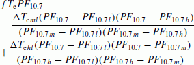  (3a)

• 2) PF_10.7 < PF_10.7l :

  

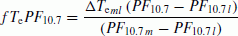  (3b)

  PF_10.7 > PF_10.7h :

  

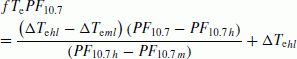  (3c)

The solar activity term, T_ePF_10.7, normalized to the solar activity of the core model can be calculated as

(4)

Full local time dependence was obtained using interpolation by harmonic function

(5)

3.3 The full model

The T_e value of the full model as each altitude and season, T_e(mlt, invdip, PF_10.7), is obtained by addition of the core model value T_e0(mlt, invdip) and of the solar activity term T_ePF_10.7(mlt, invdip, PF_10.7):

(6)

4. Model Results and Discussion

4.1 The core model

Figure 4 shows the contour plot of the core model for all five altitudes and both seasons (equinox and solstice). The model reproduces all of the well known “large scale” features of the electron temperature distribution in the topside ionosphere (see e.g. Brace and Theis, 1981; Bhuyan and Chamua, 2006; Truhlik et al., 2000, 2003; Oyama et al., 2004):

• T_e increases with altitude and the altitude gradient during daytime is much larger than during nighttime at low latitudes (±30 deg) during the nighttime the gradient reaches its lowest value.

• The morning enhancement (morning overshoot) is well developed at equatorial latitudes and at low altitudes (350, 550 to 850 km).

• The latitude dependence is more prominent at lower altitudes (350 to 850 km). Generally the lowest electron temperatures are observed close to the invdip equator. On the other hand the model does not capture small scale spatial and temporal structures like the sub-auroral electron temperature enhancement e.g. Brace (1990), the evening electron temperature crests (Balan et al., 1997) or structures in the high latitude region.

Fig. 4.

Contour plots of the main T_e model for equinox and solstice for five altitude intervals.

4.2 Comparisons with data

The performance of the model is evaluated in three ways: (i) In the first test we have calculated latitude profiles of T_e for the same conditions as in Truhlik et al. (2009a) and then we have compared these profiles with the original data-based profiles. (ii) in the second test we have used the results of the comparison of several models with data in Bilitza et al. (2007) and have added to these our new model values for comparison. (iii) In the last test we have compared the new model, and IRI Intercomos and Brace&Theis models with T_e data in our data-base.

4.2.1 Latitude profiles

Figures 5(a)/5(b) and 6(a)/6(b) show data/model latitude profiles for equinox and solstices, respectively. In each panel the medians (minimum 10 measurements are required in each bin) are plotted versus invdip latitude for low (blue), medium (green), and high (red) solar activity (called LSA, MSA, and HSA). Upper and lower quartiles are shown as error bars. In each figure each row of panels is for one of the five altitude ranges and the panels on the left are for daytime and the ones on the right are for nighttime. The model values have been calculated for the same conditions (latitude, longitude, altitude, day of year, and solar activity) as measured data.

Fig. 5. (a)

Equinox daytime (left column, MLT = 13 h ± 2.5 h) and nighttime (right column, MLT = 1 h ± 3 h) electron temperatures from our data base (median plus upper and lower quartiles) versus latitude (INVDIP) for different altitudes (1st row: 350 ± 40 km; 2nd row: 550 ± 50 km; 3rd row: 850 ± 90 km; 4th row: 1400 ±150 km; 5th row: 2000 ± 300 km) and three levels of solar activity: (a) low PF_10.7 < 110 (dashed line with triangles), (b) medium 110 ≤ PF_10.7 ≤ 180 (dash dot line with squares), (c) high PF_10.7 > 180 (solid line with circles); N_p is total number of measurements for each curve.

Fig. 5. (b)

The same as Fig. 5(a) but for T_e values calculated by the new T_e model.

Fig. 6. (a)

The same as Fig. 5(a) but for June solstice.

Fig. 6. (b)

The same as Fig. 6(a) but for T_e values calculated by the new T_e model.

The latitudinal variation shows the well-known increase of electron temperature towards higher latitudes. During nighttime in all but the highest altitude range the electron temperature is almost constant in the low and middle latitude sector (from −40 to +40 degrees).

Let us first look at the equinox plots (Figs. 5(a)/5(b)) in greater detail. Excluding the 350 and 550 km daytime cases, which will be discussed in the next paragraph, we note that for all other cases the temperature increases from LSA to MSA to HSA across all latitudes. The low altitude nighttime case (right upper panels) shows almost linear behavior. However in all other cases the solar activity variation is not always linear. At 850 km, for example, we note that the MSA and HSA curves are close together and significantly (500–1000 K) above the LSA curve. At 1400 km, on the other hand, the LSA and MSA curves are close together and well below the HSA. The model values show a little bit less range. Overall the shape of the latitudinal curves for the different levels of solar activity is very similar. An exception is the high latitude region where the large data scatter makes an interpretation much more difficult.

The most interesting behavior is seen at 350, and 550 km where the correlation with solar activity is strongly latitude dependent and becomes negative at times. With our data, which is reproduced well by the model, we find that the correlation with solar activity reverses from positive near the equator to negative at middle latitudes, to positive again at high latitudes. The anti-correlation with solar activity at mid-latitudes had been reported earlier with Incoherent Scatter Radar (ISR) observations (see references in Truhlik et al., 2009a).

Figures 6(a)/6(b) show the results for solstices (Northern summer). Data coverage did not allow plotting the complete latitudinal variations of electron temperature for high solar activity at 350 km and for low solar activity at 850 km and at 2000 km for daytime. The largest changes with solar activity are seen in the summer hemisphere (Northern hemisphere in Figs. 6(a)/(b)). Variations of T_e with solar activity are more than a factor of two larger in summer than in winter due to the increased photoelectron heating. Again we find mostly linear increase in electron temperature with increasing solar activity except for the low altitude daytime cases (350, 550 and 850 km). At 550 km we find a positive T_e response to solar activity in Summer hemisphere and a negative response in the Winter hemisphere. At 350 km the positive response is observed at in the whole range of low latitudes.

Generally, the new model reproduces the original latitude profiles surprisingly well. There is only exception at solstice 2000 km at equatorial latitudes at night. However, the original data shows very large scatter for these conditions (Fig. 6(a) lower right panel).

4.2.2 Comparison with other models and data

Figure 7(a) shows a comparison of the new T_e model with data and other models in terms of the solar activity dependence for daytime, mid-latitudes and for different altitudes and seasons. Typically, the electron temperature varies by just a few hundred degrees Kelvin. We will first discuss the behavior at 550 km. At this altitude the satellite data show a positive correlation with PF_10.7 in summer, and a negative correlation in equinox and winter. This seasonal behavior is in general agreement with the Millstone Hill model. The theoretical model (FLIP) (Bilitza et al., 2007) performs well but tends to predict a little bit higher values. The values from the new T_e model generally follow the data very well.

Fig. 7.

(a) Daytime electron temperature from our data base (mean plus standard deviation) versus solar activity for different seasons (columns) and different altitudes (1st row: 550 ± 50 km, 2nd row: 850 ± 90 km; 3rd row: 2000 ± 300 km). Also include is a least-square fitted quadratic (at 2000 km linear) approximation to the data (black curve), new T_e model (blue solid), the IRI T_e model (IK option) (blue dashed), the FLIP model (red), and the ISR averages from the Millstone Hill model (green). The green line at 2000 km (lowest row of panels) shows the temperature averages from Akebono/TED (see Bilitza et al., 2007). The orange line at 550 and 850 km (upper two rows of panels) represents the neutral temperature as given by the MSIS-86 model. The total number of data points N_p is given in the lower right of each panel. (b) Same as Fig. 7(a) but for nighttime instead of daytime electron temperature.

The plots at 850 km contain a large number of data points because this is the orbit altitude of the DMSP satellites. The FLIP model and the new T_e model represent the data quite well both in terms of the dependence on PF_10.7 and of absolute magnitude. The Millstone Hill model, on the other hand, underestimates the data and shows an increase for all seasons. This may be due to the difficulties the ISR techniques has in deducing electron temperatures in region of very low electron density.

For the plasmaspheric altitude range (2000 km) the FLIP model shows the expected increase with increasing solar activity for all seasons. The new T_e model shows the expected increase with solar activity for both solstices but for equinox it seems to indicate a “V” type dependence similar to the data averages. But the variation of the data averages is likely due to bins with rather sparse data coverage that are statistically not very reliable.

The comparison of the new T_e model with data and other models for nighttime is shown in Fig. 7(b). Temperatures generally increase with solar activity or stay constant as is to be expected from theory (e.g. in Truhlik et al., 2009b). FLIP underestimates the satellite data and the Millstone Hill model values in summer and equinox and clearly requires an additional heat source to elevate electron temperatures above the MSIS neutral temperature background. In winter heating by photoelectrons from the conjugate sunlit ionosphere helps to raise T_e above T_n and brings the FLIP temperatures closer to the satellite and radar measurements (Bilitza et al., 2007). Comparing the satellite data with the Millstone Hill model we find similar discrepancies at 850 km as were noted for daytime in the previous chapter. Unfortunately, there was not enough of data for summer at 2000 km where only one data average was available. The new T_e model values are for almost all cases in the standard deviations limit.

4.2.3 Comparison with IRI IK and Brace and Theis model

The last Fig. 8 shows predictions of three models (New T_e model, IRI T_e model IK option and IRI T_e model Brace and Theis option) versus data points for all points in low latitudes (−15° < invdip < 15°) in our database. In spite of considerable scatter (due to a natural scatter of T_e data) it can be seen that the new model shows better results than other two models.

Fig. 8.

Predictions of three models (New T_e model, IRI T_e model IK option and IRI T_e model Brace and Theis option) versus data points for all points in low latitudes (−15° < invdip < 15°) in our database. Values of corr represent the linear Paerson correlation coefficient of calculated model and measured data vectors.

5. Conclusions

A new T_e model for region from the upper ionosphere to the lower plasmasphere is presented. It represents a continuation and improvement of the previous model by Truhlik et al. (2000, 2001) but it is based on bigger volume of data and it also includes a solar activity dependence of the electron temperature based on Bilitza et al. (2007) and Truhlik et al. (2009a, b). The model is available in FORTRAN and IDL on the request from the authors.

References

Balan, N., K.-I. Oyama, G. Bailey, S. Fukao, S. Watanabe, and M. Abdu, A plasma temperature anomaly in the equatorial topside ionosphere, J. Geophys. Res., 102(A4), 7485–7492, 1997.
Bhuyan, P. K. and M. Chamua, An empirical model of electron temperature in the Indian topside ionosphere for solar minimum based on SROSS C2 RPA data, Adv. Space Res., 37(5), 897–902, 2006.
Bilitza, D., Models for the relationship between electron density and temperature in the upper ionosphere, J. Atmos. Terr. Phys., 37, 1219−1222, 1975.
Bilitza, D., International Reference Ionosphere 1990, National Space Science Data Center, NSSDC 90-22, Greenbelt, Maryland, 1990.
Bilitza, D. and W. R. Hoegy, Solar activity variation of ionospheric plasma temperatures, Adv. Space Res., 10(8), 81–90, 1990.
Bilitza, D., V. Truhlik, P. G. Richards, T. Abe, and L. Triskova, Solar cycle variations of mid latitude electron density and temperature: Satellite measurements and model calculations, Adv. Space Res., 9(5), 779–789, 2007.
Brace, L. H. and R. F. Theis, Global empirical models of ionospheric electron temperature in the upper F-region and plasmasphere based on in situ measurements from atmosphere explorer C, ISIS-1 and ISIS-2 satellites, J. Atmos. Terr. Phys., 43, 1317–1343, 1981.
Brace, L., Solar cycle variations in F-region Te in the vicinity of the midlatitude trough based on AE-C measurements at solar minimum and DE-2 measurements at solar maximum, Adv. Space Res., 10(11), 83–88, 1990.
Evans, J. V., Seasonal and sunspot cycle variations of F Region electron temperatures and protonospheric heat fluxes, J. Geophys. Res., 78(13), 2344–2349, 1973.
Köhnlein, W., A model of the electron and ion temperature in the ionosphere, Planet. Space Sci., 34, 609–630, 1986.
Mahajan, K. K. and V. P. Pandey, Solar activity changes in the electron temperature at 1000-km altitude from the Langmuir probe measurements on ISIS 1 and Explorer 22 satellites, J. Geophys. Res., 84, 5885–5889, 1979.
Martinec, Z., Program to calculate the least-squares estimates of the spherical harmonic expansion coefficients of an equally angular-gridded scalar field, Comput. Phys. Commun., 64, 140–148, 1991.
Oyama, K.-I., P. Marinov, I. Kutiev, and S. Watanabe, Low latitude model of Te at 600 km based on Hinotori satellite data, Adv. Space Res., 34(9), 2004–2009, 2004.
Richards, P. G., J. A. Fennelly, and D. G. Torr, EUVAC: A solar EUV flux model for aeronomic calculations, J. Geophys. Res., 99(A5), 8981–8992, 1994.
Sharma, P. K., P. P. Pathak, D. K. Sharma, and J. Rai, Variation of ionospheric electron and ion temperatures during periods of minimum to maximum solar activity by the SROSS-C2 satellite over Indian low and equatorial latitudes, Adv. Space Res., 45(2), 294–302, 2010.
Titheridge, J. E., Temperatures in the upper ionosphere and plasmasphere, J. Geophys. Res., 103(A2), 2261–2277, 1998.
Truhlik, V., L. Triskova, J. Smilauer, and V. V. Afonin, Global empirical model of electron temperature in the outer ionosphere for period of high solar activity based on data of three Intercosmos satellites, Adv. Space Res., 25(1), 163–169, 2000.
Truhlik, V., L. Triskova, and J. Smilauer, Improved electron temperature model and comparison with satellite data, Adv. Space Res., 27(1), 101–109, 2001.
Truhlik, V., L. Triskova, and J. Smilauer, Response of outer ionosphere electron temperature and density to changes in solar activity, Adv. Space Res., 31(3), 697–700, 2003.
Truhlik, V., D. Bilitza, and L. Triskova, Latitudinal variation of the topside electron temperature at different levels of solar activity, Adv. Space Res., 44(6), 693–700, 2009a.
Truhlik, V., L. Triskova, D. Bilitza, and K. Podolska, Variations of daytime and nighttime electron temperature and heat flux in the upper ionosphere, topside ionosphere and lower plasmasphere for low and high solar activity, J. Atmos. Sol.-Terr. Phys., 71(17–18), 2055–2063, 2009b.
Webb, P. A. and E. A. Essex, Modifications to the Titheridge upper ionosphere and plasmasphere temperature model, J. Geophys. Res., 108(A10), 1359, doi:10.1029/2002JA009754, 2003.
Acknowledgments
We are very grateful to K.-I. Oyama, J. Smi-lauer, M. Hairston, F. Rich, K. W. Min and P. K. Bhuyan for providing data from Hinotori, Intercosmos (19, 24, 25), DMSP (F12, F13, F14, and F15), DMSP (F10 and F11), KOMPSAT-1 and SROSS C2 satellites, respectively. We are also grateful to NASA’s National Space Science Data Center (NSSDC) and Space Physics Data Facility (SPDF) for providing the other satellite Te data and also the Modelweb interface. We also thank Katerina Podolska, BSc., employee of the Institute of Atmospheric Physics for help with processing of the huge amount of DMSP data. This study was supported by grant A300420603 of the Grant Agency of the Academy of Sciences of the Czech Republic, by grant P209/10/2086 of the Grant Agency of the Czech Republic and by NASA grant NNH06CD17C.
Author information
Authors and Affiliations
Corresponding author
Rights and permissions
Open Access This article is licensed under a Creative Commons Attribution 4.0 International License, which permits use, sharing, adaptation, distribution and reproduction in any medium or format, as long as you give appropriate credit to the original author(s) and the source, provide a link to the Creative Commons licence, and indicate if changes were made.
The images or other third party material in this article are included in the article’s Creative Commons licence, unless indicated otherwise in a credit line to the material. If material is not included in the article’s Creative Commons licence and your intended use is not permitted by statutory regulation or exceeds the permitted use, you will need to obtain permission directly from the copyright holder.
To view a copy of this licence, visit https://creativecommons.org/licenses/by/4.0/.
About this article
Cite this article
Truhlik, V., Bilitza, D. & Triskova, L. A new global empirical model of the electron temperature with the inclusion of the solar activity variations for IRI. Earth Planet Sp 64, 531–543 (2012). https://doi.org/10.5047/eps.2011.10.016
Received:
Revised:
Accepted:
Published:
Issue Date:
DOI: https://doi.org/10.5047/eps.2011.10.016