Diagnosing low earth orbit satellite anomalies using NOAA-15 electron data associated with geomagnetic perturbations

Abstract

A satellite placed in space is constantly affected by the space environment, resulting in various impacts from temporary faults to permanent failures depending on factors such as satellite orbit, solar and geomagnetic activities, satellite local time, and satellite construction material. Anomaly events commonly occur during periods of high geomagnetic activity that also trigger plasma variation in the low Earth orbit (LEO) environment. In this study, we diagnosed anomalies in LEO satellites using electron data from the Medium Energy Proton and Electron Detector onboard the National Oceanic and Atmospheric Administration (NOAA)-15 satellite. In addition, we analyzed the fluctuation of electron flux in association with geomagnetic disturbances 3 days before and after the anomaly day. We selected 20 LEO anomaly cases registered in the Satellite News Digest database for the years 2000–2008. Satellite local time, an important parameter for anomaly diagnosis, was determined using propagated two-line element data in the SGP4 simplified general perturbation model to calculate the longitude of the ascending node of the satellite through the position and velocity vectors. The results showed that the majority of LEO satellite anomalies are linked to low-energy electron fluxes of 30–100 keV and magnetic perturbations that had a higher correlation coefficient (~ 90%) on the day of the anomaly. The mean local time calculation for the anomaly day with respect to the nighttime migration of energetic electrons revealed that the majority of anomalies (65%) occurred on the night side of Earth during the dusk-to-dawn sector of magnetic local time.

Introduction

Placing a satellite into space is a challenge owing not only to the technical aspects of the mission requirements but also because of the space environment of the satellite placement and operation. The variability of the space environment around the satellite can lead to multiple effects such as loss of performance in satellite subsystems. Although some effects present low-level and temporary risks from which the satellite can recover, others present high-level risks that can result in notorious failures that can permanently stop the satellite operation. The reliability of satellites is tested and proved well before launch to avoid damage during operation; nevertheless, failures arise owing to many factors such as command errors, mechanical and electrical faults, and design or manufacturing problems as well as environmental effects on the satellite (Vampola 1994).

The causes of satellite failures are generally difficult to diagnose accurately; thus, they are often referred to as anomalies. Documentation of numerous anomaly cases and knowledge about the proximate causes has led to an understanding that plasma variation around satellites also plays an important role in anomalies through interaction between the plasma and satellite system. This interaction gives rise to various impacts on satellites depending on satellite orbit, relative position in space, satellite local time (SLT), solar and geomagnetic activities, and materials in the satellite structure (Hastings and Garret 1996).

It is believed that satellite anomalies occur predominantly during periods of high geomagnetic activity, which can change the plasma properties abruptly and accelerate electrons and ions to energies on the order of kiloelectronvolts. Electrons and ions with energies above tens of kiloelectronvolts are known to contribute greatly to spacecraft charging phenomena (Lai 2012). Because the thermal speed of electrons is much larger than that of ions, the electron impact on satellites is of prime interest for satellite anomaly diagnosis, especially in low Earth orbit (LEO) environments below an altitude of 1000 km.

Regarding LEO satellites, the effects of charging by plasma variation are not critical except in some regions such as polar regions and a small equatorial region known as the South Atlantic Anomaly. Plasma in those regions is cold and dense with typical energies less than 10 keV, although it can change rapidly during periods of high geomagnetic activity. Rapid changes in plasma properties around a satellite can be problematic for some sensors and even for the satellite itself through charging effects. Plasma variations in LEO can be destructive because the collective plasma can release sufficient energy to the satellite to cause effects such as surface charging, detector contamination, and surface chemical reactions (Hastings 1995). Of interest is that satellite charging occurs in finite time until an equilibrium state is reached (Lai 2012). Moreover, the current balance on a satellite owing to its interaction with plasma depends strongly on material properties as well as the flux of energetic particles along the satellite trajectory.

One of the challenges in diagnosing satellite anomalies arises from the limited amount of anomaly data because some anomalies have not been formally or thoroughly documented (Koons et al. 2000). In addition, it is difficult to maintain a comprehensive database in which all anomalies are categorized by, for example, satellite orbit type, material properties, position on the anomaly day, SLT, type of anomaly, and space weather at the time of the anomaly. In addition, the database should contain detailed descriptions of anomalies, including the initial presumption of cause, and it should be up to date.

Numerous studies have been published regarding satellite anomaly events, including the estimation of causes, but the majority of research is more concerned with geosynchronous Earth orbit (GEO) satellites; few studies have examined anomalies in LEO and medium Earth orbit satellites (Fennell et al. 2001; Belov et al. 2005; Pilipenko et al. 2006; Iucci et al. 2006; Patil et al. 2008; O’Brien 2009; Choi et al. 2011; Thomsen et al. 2013). In addition, in the attempt to find anomaly causes related to environmental change, most analyses have used high-energy particle data at energies on the order of megaelectronvolts for both electrons and protons.

It is a challenge to study anomaly cases for satellites in the LEO environment because they were the most numerous among active satellites in 2015, with a total of 696 (53.33%), whereas satellites in GEO numbered about 481 (36.86%; UCS 2015). That is, the population of LEO satellites is significantly higher than that of GEO satellites (SIA 2015).

In this study, we undertook the diagnosis of the proximate causes of anomalies on LEO satellites recorded on the Satellite News Digest website (SND 2017) and evaluated their relationship with space environment variations during a specific period before and after the anomaly. The space environment was obtained primarily from low-energy electrons detected by the National Oceanic and Atmospheric Administration (NOAA)-15 satellite (NOAA NCEI 2017) as well as by geomagnetic parameters represented by two indices: Kp and Dst (NASA GSFC 2016). To acquire the SLT, an important factor for anomaly diagnosis, we applied the Simplified General Perturbation-4 (SGP4) code to two-line element (TLE) data for each satellite obtained from Space-Track (2015). All of these steps enabled us to diagnose the relationship between low-energy electron fluxes and their associated magnetic perturbations with regard to their effect on LEO satellites.

Data and method

NOAA-15/MEPED electron data

The NOAA-15 satellite was launched on May 13, 1998, and was placed at an altitude of 807 km with a polar inclination of around 98.8°. This satellite is equipped with Space Environment Monitor 2 instruments including the Medium Energy Proton and Electron Detector (MEPED), which is a set of solid-state energetic particle detectors that measure the flux of protons and electrons within an energy range of 30 keV to 200 MeV. To measure particles from different directions, the detectors are orientated in the zenith (0°) and horizontal/perpendicular-to-zenith (90°) directions and are referred to here as the 0° and 90° detectors, respectively. The MEPED also has omnidirectional detectors (Evans and Greer 2004), although these data were not used in the present study. The MEPED instrument measures only the electron fluxes in three energy channels that span 30–2500 keV. Because the electron detectors are also sensitive to protons, as shown in Table 1, all electron data must be examined and corrected to obtain better accuracy.

Table 1 MEPED electron energy channel detection and proton contamination ranges

Table 1 shows the proton energy ranges at which each electron channel is subject to contamination by protons (CP) with an energy range of 210–2700 keV for E1 channel. The E2 electron channel is sensitive to protons over the energy range of 280–2700 keV; and the E3 channel is affected by protons in the range of 440–2700 keV (Evans and Greer 2004). Protons with energies in these ranges contaminate the electron detector channels and affect electron flux measurement; thus, their effects must be removed from the data. Several methods can remove CP from electron data, as introduced by Lam et al. (2010), Rodger et al. (2010), Asikainen and Mursula (2013), and Peck et al. (2015). Because we used only short-term data over the 7 days straddling the anomaly day, the electron data were examined by comparing the flux variations between electrons and the CP within specific intervals, as done by Tadokoro et al. (2007). When the trend of electron fluxes differed from the proton fluxes, the electron data were regarded as contaminant-free. Furthermore, we also adopted the method introduced by Rodger et al. (2010), in which the electron data are deemed to have acceptable quality if the electron flux in each energy channel is larger than twice the CP flux. We applied these methods for removing CP from electron channels for some anomaly cases, as shown in Fig. 1.

Fig. 1

Variation of electron and proton fluxes during the 7-day interval straddling the anomaly day on a ASCA, b FUSE (1), c ERS-1, and d Radarsat-1(1). The red, blue, and green curves represent electron fluxes for channels E1, E2, and E3, respectively, and the black and light blue curves indicate the variation of contaminating protons obtained from methods 1 and 2 in sequence

In the present study, we focus on the variation of electron flux during the 7-day interval straddling the anomaly day for four cases: two equatorial satellites, ASCA and FUSE (1), and two polar satellites, ERS-1 and Radarsat-1(1). The other 16 cases are presented in the “Appendix”. We used the hourly averages of electron flux to match the magnetic field data. Figure 1 shows the electron flux variations for channels E1 (red lines), E2 (blue lines), and E3 (green lines). The trend of CP on the electron fluxes is indicated by the black lines. Overall, the protons affected only a small portion of the electron flux data: day of year (DOY) 197-198 for ASCA (Fig. 1a) and DOY 328-329 for FUSE (1) (Fig. 1b) for both the 0° and 90° detectors. Significant CP was not found in the other two cases (Fig. 1c, d) in channel E1, whereas CP significantly affected the electron data in channels E2 and E3. It should be noted that CP did not occur exactly in conjunction with the increase in electron flux: The pattern of the peaks was totally divergent. The average CP in the electron channels was obtained from the following formula:

$$\frac{{\bar{\varGamma }_{p} }}{{\bar{\varGamma }_{e} }} \times 100\% \approx {\text{CR}}$$

where $\bar{\varGamma }_{p}$ and $\bar{\varGamma }_{e}$ are the average flux of protons and electrons, respectively, within the selected interval, and CR is the percentage of proton flux contamination in the electron channels. The rates of CP for the same four anomaly cases are shown in Table 2.

Table 2 Proton contamination in each energy channel as a percentage of electron fluxes within ± 3 days of the anomaly day for each case

The biggest CP occurred in channel E3 for both detectors and all cases. A higher energy corresponded to a larger CP. Moreover, it appears that the magnitude of contamination is independent of satellite orbit. The data from both equatorial and polar satellites showed similar magnitudes of CP.

To confirm that the electron data were usable, the second method was applied. The electron fluxes in each energy channel should be larger than twice the CP, hereafter referred to as 2CP, because one contaminant will result in one incorrect electron flux (Rodger et al. 2010). The 2CP values are indicated by the light blue curves in Fig. 1. Only electrons in channel E3 for both the 0° and 90° detectors were affected by CP. The increases in electron flux were followed by proton flux enhancement with similar patterns. The other channels, E1 and E2, were not totally affected by the contaminant. Based on this confirmation of usability, we removed the CP from the electron data using the aforementioned methods.

Particle data from the 0° and 90° detectors were used in this study for the following reasons. When the NOAA-15 satellite passes through a high-latitude region, the 0° detector measures precipitated particles, whereas the 90° detector counts trapped particles. Conversely, during low-latitude passage, the 0° detector measures trapped particles, whereas the 90° detector counts precipitated particles (Asikainen and Mursula 2008). Owing to the orthogonal orientation of the detectors, we attempted to reconcile the electron data from both detectors to simplify the diagnosis process. In this study, reconciliation was performed by using the following steps. First, hourly averages of electron data were selected from the 0° and the 90° detectors. Second, the CP was removed from all electron channels in both detectors by deducting or subtracting the proton fluxes from the electron flux data. This subtraction was appropriate because one flux of contaminant will produce one incorrect electron flux (Rodger et al. 2010). This means that the presence of proton flux in the electron detector will lead to incorrect measurement of electron flux; thus, it needs to be removed. In most cases, the electron fluxes were twice the size of the CP fluxes except for channel E3, indicating the domination of electron flux in the electron detector. Because we used only short intervals of 7 days, the trend lines showed that the contaminant affected only a small portion of the electron data, such as on DOY 197-198 and DOY 328-329 in Fig. 1a, b, respectively. Thus, not all electron data during the selected interval were contaminated significantly by protons, as shown in Fig. 1. Third, we calculated the magnitude or result of the corrected electron flux data from the second step: $\varGamma_{\text{corr}} = {\text{sqrt(}}\varGamma_{{0\deg \;{\text{corr}}}}^{2} + \varGamma_{{90\deg \;{\text{corr}}}}^{2} )$, where $\varGamma_{{0\deg \;{\text{corr}}}}$ and $\varGamma_{{90\deg \;{\text{corr}}}}$ are corrected electron fluxes from the 0° and 90° detectors, respectively. These data were used with the magnetic field data to diagnose the anomalies on the LEO satellites.

Kp and Dst indices as diagnosis parameters

Geomagnetic data provide fundamental parameters for environmentally induced satellite anomaly research. These data, along with the energetic particle data, have been used to diagnose anomalies on LEO and GEO satellites. In this study, we used only the geomagnetic data represented by the Kp and Dst indices because these data have shown good agreement with anomaly events, as reported by Belov et al. (2005 ), Patil et al. (2008), and Choi et al. (2011).

The Kp index is an indicator of global geomagnetic disturbance counted by a scale of 0 to 9. In general, a larger Kp index corresponds to more anomaly occurrences. Farthing et al. (1982) showed that anomalies on the GOES satellite series are clearly linked to Kp index values ranging from 1 to 6. Their finding showed that the overall tendency of anomalies increased with higher Kp. Fennell et al. (2001) also found that highly elliptical orbit satellite anomalies increased with an increase in Kp. Furthermore, Choi et al. (2011) found that although some GEO satellite anomalies were linked to lower Kp values, the number of GEO anomalies increased with an increase in Kp.

The level of geomagnetic disturbance can also be indicated by the Dst index, which quantifies plasma changes in the ring current owing to those disturbances. During magnetic storms, the Dst index drops rapidly as the energetic electron flux increases substantially (Fennell et al. 2001). Several studies, such as Belov et al. (2005), pointed out that a numerous satellites in different groups are linked to magnetic storms through the Dst index. Pilipenko et al. (2006) also found a similar relationship between GEO anomalies registered in the National Geophysical Data Center databases in conjunction with Dst index variation. They noted that not all anomalies occurred precisely at the time of significant drop in the Dst index.

In this study, a Dst index less than − 30 nT (Gonzales et al. 1994) and a Kp index in the range of 3 to 9 indicated a high level of geomagnetic activity. Such high levels are generally associated with geomagnetic storms and substorms. In some events, a geomagnetic substorm occurs during the main storm phase (Wu et al. 2004) and can lead to partial ring current formation (Gonzales et al. 1994). The use of these bounds in the present study is intended to simply identify the levels of geomagnetic activity regarding anomaly occurrences. We also adopted an interval of 3 days before the anomaly day because Choi et al. (2011) found that such an interval has good agreement with the occurrence rate of the anomalies. We appended the interval of 3 days to examine the characteristic environment after the anomaly day. Charged particles can remain in the satellite orbital path during the recovery phase of magnetic storms (Choi et al. 2011). Although Choi et al. (2011) focused on GEO satellites, we found similar features in LEO (“Results and discussion” section).

SND database of anomalies

Numerous studies, such as Robertson and Stoneking (2003) and Belov et al. (2005), have examined anomalies on LEO satellites using various databases. The former study used only a small number of LEO anomaly cases, whereas the latter study applied Kosmos data on anomalies attributed to high-energy particles. It is difficult to inventory the LEO satellite anomaly data exhaustively because most anomalies are not very accessible. In this study, we used only SND data but excluded some failures attributed to space debris. Moreover, we rechecked and confirmed some SND data in terms of anomaly date and failure descriptions by using other sources, and the appropriate adjustments were made.

Failure descriptions provided by the SND can be the initial step for anomaly diagnosis. The descriptions contain information about failure status, such as partial loss, total loss, or contact loss, as well the satellite subsystem sustaining damage, such as solar array failure, power drop, or reaction wheel failure. Failure descriptions, along with the anomaly time, were used to construct the criteria to select the LEO satellites for analysis. As criteria used in this analysis, all failures owing to space debris were ignored. In addition, satellites were used only if the difference between the perigee and apogee of their orbit was less than 100 km or if their orbital eccentricity was almost circular. As a result, all LEO anomaly cases in this study involve satellites having orbits similar to that of the NOAA-15 satellite, which assures the relevance of the electron data used in this study.

It should be noted that not all sources of LEO satellite failure used in this study were explicitly stated; thus, we presumed that the anomalies with unknown causes are associated with plasma variations triggered by geomagnetic disturbances. This is consistent with other studies that attributed anomalies to environmental changes by default when analysis from telemetry data was infeasible (Vampola 1994; Gubby and Evans 2002). The LEO satellite anomaly cases used in this paper are listed in Table 4.

Some information in Table 4, such as altitude and inclination, are somewhat different from the existing data in SND. We preferred to use satellite orbital data from Space-Track because it also provided the TLE data used for SLT calculation for each satellite. As previously mentioned, we attempted to confirm the anomaly day for each satellite and found that only the ICESat anomaly day had a discrepancy. ICESat was reported to suffer failure on March 29, 2003, around 9:58 a.m. Eastern Standard Time (EST), when the Geoscience Laser Altimeter System transmitter stopped emitting laser pulses (Kichak 2011). Hence, in this study, we preferred to use the date reported by the National Aeronautics and Space Administration (NASA) for the ICESat anomaly. All other anomaly days were obtained from the SND database. We also found that two satellites, FUSE and Radarsat-1, incurred anomalies more than once. Therefore, the first anomalies were designated as FUSE (1) and Radarsat-1(1), and the second were FUSE (2) and Radarsat-1(2).

Results and discussion

Relationship between electron flux and magnetic flux

We initially examined the strengths of geomagnetic disturbances affecting the properties of plasma in space. A previous study showed that the charge buildup on satellites as a trigger of anomalies did not originate from the magnetic perturbations but rather from energetic electrons affecting the satellite surfaces (Lam and Hruska 1991). The properties of energetic particles and plasma around Earth change in association with magnetic perturbations. In addition, some studies have shown that lower-energy electrons of <100 keV have fluctuated more strongly with geomagnetic variability compared with higher-energy electrons (Pilipenko et al. 2006; Choi et al. 2011). The first study used the Dst index in association with electron fluxes of >1 MeV and >2 MeV, whereas the latter applied the Kp index corresponding to electron fluxes of 50 keV to 1.5 MeV. Because the magnetic perturbations are believed to be indicative of plasma changes in space, we examined the relationship between both indices together with electron flux variations within the 7-day interval. We first evaluated the relationship of Kp, Dst, and electron flux in each detector energy channel (E1, E2, and E3) and then identified the energy channel most strongly associated with magnetic perturbations represented by both indices. It should be noted that the electron fluxes from all three channels have the same number of datasets for each event. Because we can access all magnetic data from NASA GSFC (2016), we preferred to use the hourly averaged data for Kp and Dst and to adjust the 1-h resolution for electron flux data to match the resolution of the selected Kp and Dst data. The relationship of each energy channel is expressed by a correlation coefficient, designated as R, which is shown in Fig. 2 for the same four anomaly cases as those given in Fig. 1.

Fig. 2

Relationship of geomagnetic variability (Kp and Dst indices) and electron fluxes for channels E1 (left), E2 (middle), and E3 (right) around the day of anomaly for a ASCA, b FUSE (1), c ERS-1, and d Radarsat-1(1). The red and blue spots indicate the relationship with Kp and Dst data, respectively

Because we adopted the seven-day interval, which is essentially short-term data, the images in Fig. 2 were created by averaging all data points (Dst and E1, E2, and E3 data) corresponding to various Kp bins at intervals of 10: 0, 10, 20, …, 90. We then fitted the line for the averages of the bins rather than for the entire dataset. The red (blue) spots in the figure represent a scatter diagram for the averaged Kp (Dst) index bins. The R values of each energy channel are given at the top and bottom of each panel. The R values show that the electrons with lower energy (E1) obviously have a stronger relationship with magnetic perturbations than those with higher energy (E2 and E3). This strong correlation was evident for both Kp and Dst indices. Overall, the R values for channel E1 were larger than those for channels E2 and E3. In this study, the Kp index value was multiplied by 10 (Kp × 10) for scaling purposes.

We initially expected that the correlation would be significantly higher during the period of solar maximum in 2000 and 2001 because the electrons trapped in the magnetosphere are related to solar activity (Lam et al. 2010). The anomalies ASCA, FUSE (1), and ERS-1 (Fig. 2a–c, respectively) occurred during the solar maximum. Geomagnetic disturbances occurred several times, as indicated by the Kp and Dst indices. For the anomalies in these three satellites, the maximum Kp index values were 9, 8.3, and 4.3, respectively, whereas the Dst index dropped to − 300, − 221, and − 51 nT, respectively. We presumed that the relationship was not always individually consistent for every event owing to the different datasets. Furthermore, high-level geomagnetic disturbances were not always followed by increased electron flux. A plausible explanation for the time lag between geomagnetic disturbance and electron flux enhancement ranging from hours to days is that it is driven by a mechanism such as radial transport diffusion or pitch-angle scattering (Tadokoro et al. 2007). However, the overall trend for each anomaly case showed that lower-energy electrons (>30 keV, channel E1) had a good correlation with Kp and Dst values, as shown in Fig. 3.

Fig. 3

Correlation coefficient between electron fluxes and (left) Kp index and (right) Dst index for channels E1 (red), E2 (blue), and E3 (light blue) for selected cases

In Fig. 3, the x-axes represent a sequence of seven of the satellite anomaly cases listed in Table 4. Because the FUSE (2) and Yohkoh anomalies occurred within 5 days of each other, we merged their data for simplicity. Hence, in the diagnosis steps, both satellites were designated as Additional file 1: case #5, using #5a for FUSE (2) and #5b for Yohkoh. In general, the correlation trend was consistent for each anomaly case, where R for E1 was larger than that for E2 and E3. Furthermore, the right-hand panel shows a correlation with the Dst index, where for some cases the level of disturbance was less than − 100 nT (intense storm), such as in case #4 (Fig. 4b). For some events, such as Additional file 2: case #14, no storm was present. We also noted that electron flux had a negative correlation with Dst because the ring current energy containing electrons and ions is inversely proportional to the magnitude of Dst (Lohmeyer et al. 2012). Overall, the trend in Fig. 3 shows that the majority of lower-energy electrons are highly responsive to geomagnetic disturbance. Hence, in the following section, we diagnosed LEO satellite anomalies using only lower-energy electron data (channel E1).

Diagnosis of LEO satellite anomalies

Satellite failure descriptions can provide clues for tracing the source of anomalies. The SND data used in this study did not contain any assertive statements to definitively identify the cause of any anomalies. In addition, our investigation to find the relationship between LEO anomalies and environmental changes was hindered by the limited amount of data. For example, we obtained only five anomaly cases for equatorial satellites, whereas the remaining cases involved polar satellites. Furthermore, the majority of anomalies were presented as technical failures, such as attitude loss and power drop, without identifying the cause of those conditions, such as environment, debris, or phantom command. The descriptions are summarized below.

• ERS-1 operated for almost nine years before being terminated by the European Space Agency owing to failure in its attitude control system (ACS); no report about the cause of the ACS failure was prepared.

• ASCA (Astro-D) lost its attitude, and a power drop coincided with increased solar activity. Increasing incident solar radiation was suspected to impart torque to the satellite, which increased its drag. Atmospheric drag strongly affects satellite orbit, rather than onboard systems, so we concluded that the cause of this anomaly remains unknown.

• FUSE was reported to experience several reaction wheel failures in quick succession. Although it initially recovered, the third and fourth reaction wheels incurred damage several times until they failed completely in August 2007. No explanation of the failure cause is available.

• Radarsat-1 was discontinued by the Canadian Space Agency owing to a deteriorating ACS. This satellite had previously incurred excessive friction and temperature in the primary momentum wheel in September 1999. Its back-up wheel had a similar problem in November 2002. No information about the cause of the anomaly is available.

• Midori-2 (ADEOS-2) switched to “light load” mode owing to an unknown anomaly. The power level fell from 6 kW to 1 kW. It was presumed that a relationship might exist between the accident and solar flares. Further investigation is needed.

• No definite information was available on the causes of failure for satellites in the SND database (SND 2017) other than those detailed in this paper; therefore, further study is needed.

Because we were unable to obtain much conclusive information about the causes of anomalies from the SND database or other sources (http://www.astronautix.com and http://spaceflight101.com/spacecraft/satellite-catalog), we attributed these anomalies to environmental changes by default. As the first step, we traced the changes in environmental conditions using the Kp and Dst indices as well as the electron flux data from channel E1, as shown in Fig. 4.

Fig. 4

Variation of electron fluxes and geomagnetic disturbances during the 7-day interval straddling the anomaly day for a ASCA, b FUSE 1(1), c ERS-1, and d Radarsat-1(1). The red, blue, and green curves are the Kp index, Dst index, and electron flux in channel E1, respectively

In the figure, the left y-axes represent the magnitude of geomagnetic disturbance for both the Kp (red curves) and Dst indices (blue curves), whereas the right y-axes designate the electron fluxes for channel E1 (green curves). As previously discussed, the lower-energy electrons (E1) correlated significantly to magnetic perturbations. The interval inside the black dashed lines indicates the day on which the anomaly occurred. The first two panels (Fig. 4a, b) show data for equatorial satellites (ASCA and FUSE (1)), whereas the last two panels (Fig. 4c, d) show data for polar satellites (ERS-1 and Radarsat-1(1)).

It is of interest that the “peaks” of Kp and “valleys” of Dst did not occur simultaneously owing to their different complex mechanisms. A time lag existed sometimes between two events. For example, in Fig. 4a, the magnetic activity increased 2 days prior to the anomaly day (DOY 195), although a decline in Dst (down to -43 nT) was preceded by an increase in Kp (up to 6.3). We also found this pattern in other cases, as described in the “Appendix”. The Kp index globally measures the magnetic activity at high geomagnetic latitudes in which plasma in the magnetotail is heated and is then transported earthward, whereas the Dst is measured at low latitudes linked to ring current disturbances. We attributed the time lag to differences in the observation method. In addition, the differences could be related to the transport mechanism in which the energetic particles are first accelerated at high latitudes and are then transported to drift into the ring current (Prolss 2004). The transport mechanism likely leads to measurement time lags between Kp and Dst. The existence of a time lag between Kp and Dst, especially at the peak of geomagnetic disturbances, affects the identification of satellite anomaly occurrences in association with Kp enhancement and Dst depression simultaneously. In some events, the anomaly had good correlation with Kp, as shown in Additional file 1: case #5b (Yohkoh; “Appendix”), whereas other events showed that the anomaly was related to Dst, as in case #4 (FUSE (1), Fig. 4b). Thus, the use of both indices in this paper increased our ability to associate anomalies with geomagnetic phenomena.

Previous attempts to link anomalies to magnetic activity, such as Fennell et al. (2001), showed that the majority of anomalies occurred during substorms, although not all substorms led to anomalies. During a geomagnetic substorm, a numerous energetic particles driven by solar wind interact with local plasma in the geomagnetic tail on the night side of Earth, resulting in plasma configuration changes. The increased plasma energies from this process are injected toward Earth through plasma sheets. Any satellites that cross these regions potentially experience charge buildup. Moreover, it is well established that an increase in particle flux associated with magnetic activity occurs during a period of increasing anomalies (Welling 2010), although only 15% of anomalies occurred during magnetically disturbed conditions. In this study, we investigated the LEO satellite anomalies listed in Table 4 according to three patterns:

• 1. The anomaly coincided with the main phase of a magnetic storm (pattern 1).

• 2. The anomaly occurred during the recovery phase of a magnetic storm (pattern 2).

• 3. High geomagnetic activities occurred during the 3 days before or after the anomaly day (pattern 3).

These patterns were used in the present study to evaluate anomalies on LEO satellites. However, only 60% of anomalies (12 cases) fit one of the three patterns; 40% (8 cases) showed weak correlation to magnetic variability. For the ASCA, FUSE (1), ERS-1, and Radarsat-1(1) anomalies in Fig. 4, we found that all the above criteria were satisfied by these cases collectively because magnetic storms followed by an increase in electron flux occurred prior to and up to the anomaly day. In Fig. 4a (ASCA), a magnetic storm began on DOY 195 (Kp 7 and Dst − 43 nT). It is clear that electron flux enhancement occurred gradually following the increase in Kp (~9) and decrease in Dst (~ − 289 nT) on the anomaly day (DOY 197). This occurred during the main phase of a magnetic storm (pattern 1). We did not observe a significant time lag during this event; thus, we concluded that the activity was caused likely by the mechanism explained by Gonzales et al. (1994), in which a large injection of energetic particles from the magnetotail into the ring current and high-latitude region is proportionally constant. Moreover, the increased electron flux affected ASCA on the anomaly day, which coincided with the increase in Kp and decrease in Dst.

In contrast to the ASCA case, case #4 (FUSE (1), Fig. 4b) appears to have different features, in which the anomaly occurred during the recovery phase of a magnetic storm (pattern 2). The disturbance of geomagnetic field strength occurred a few days prior to the anomaly day and was severe on DOY 328, which is 1 day before the FUSE (1) anomaly day. The maximum Kp was 8.3, and the minimum Dst was − 221 nT on DOY 328. We found that the time lag between the Kp and Dst changes was insignificant, as in the ASCA case. Therefore, we presumed that energetic electrons were accelerated in the magnetotail plasma sheet and were then transported into the ring current. The insignificant time lag between Kp and Dst changes for the ASCA and FUSE (1) anomalies confirm that both indices had good agreement with electron flux enhancement during periods of highly disturbed geomagnetic activity. We also found this pattern in other cases, such as Additional file 3: cases #12 (DART) and Additional file 4: cases #13 (Monitor-E; “Appendix”). Although FUSE is an equatorial satellite and the other two satellites (DART and Monitor-E) are polar satellites, it appears that pattern 2 is independent of satellite orbit.

Pattern 3 was found in the ERS-1 anomaly (Fig. 4c), where multiple storms occurred around the anomaly day. The strongest, on DOY 68 (Kp 4 and Dst − 51 nT), weakened to a similar maximum Kp but lower Dst strength (~ − 35 nT) on the anomaly day (DOY 70). In general, the electron flux fluctuated in step with the Kp variation, indicating that electron streams were injected earthward from the magnetotail and reached LEO with temporal fluctuation. For the Radarsat-1(1) anomaly in Fig. 4d, several magnetic storms also occurred on DOY 329 (Kp 3.7 and Dst − 60 nT) and became stronger on the anomaly day (Kp 5 and Dst − 64 nT). A similar pattern was found in other cases, such as Terra (#3), Yohkoh (#5b), Radarsat-1(2) (#8), Landsat 7 (#9), ICESat (#10), and Midori (#11; “Appendix”). Most LEO anomalies in this study are associated with pattern 3.

It is interesting that no anomalies occurred prior to the reported anomaly day because several magnetic storms obviously occurred before that day, as shown in Fig. 4 and in the “Appendix”. To explain this phenomenon, we propose the following scenarios.

• 1. Anomalies occurred with a time delay between storm occurrence and incoming electrons near the satellite, as shown in Fig. 4b, c. This was also found in some anomaly cases studied by Farthing et al. (1982), Lam and Hruska (1991), and Iucci et al. (2006 ).

• 2. The link between LEO anomalies and environmental change was weak in some cases, specifically #5a [FUSE (2)], #6 (Aqua), and from case #14 (Kirari) to case #19 (Orbcomm) in Table 4 (Additional files 2, 11, 12, 13, 14, and 15) in Appendix. Weak linkage was also found in GEO anomaly cases studied by Gubby and Evans (2002).

• 3. Anomalies were not promptly logged and documented by the satellite operator when the anomaly occurred. The anomaly occurrence was logged and documented several days after the event, resulting in an inaccurate local time for the anomaly. This evidence was found by one of the authors during analysis of some anomaly cases using unpublished data from a satellite operator.

As another interesting point, we found that some anomalies occurred on the cuspate gradients, where the curve of electron flux and Kp and Dst indices change steeply. This feature was also found by Gubby and Evans (2002). In Fig. 4a, the sharp drop in Dst on DOY 197 indicates an abrupt change in electron streams, especially in the ring current. The electron flux fluctuated rapidly during this period. A similar pattern is shown in Fig. 4c on DOY 70 and in Fig. 4d on DOY 331. Contrary to these cases, Dst in Fig. 4b shows a clear cuspate gradient on DOY 328 that was followed by increased electron flux. However, the impact on FUSE (1) was delayed. Because several storms occurred prior to the anomaly day, it is still problematic to precisely determine which pattern contributed to the anomaly.

It remains unknown which energies are primary contributors to satellite anomalies (Choi et al. 2011). Generally, however, the use of the lower-energy channel (30–100 keV, channel E1) is relevant in this study owing to its sensitivity to geomagnetic disturbances, as demonstrated by the R values presented in Fig. 2.

To support this relationship, we adopted a method used by Choi et al. (2011) to calculate the anomaly occurrence rate for LEO satellites. We selected the maximum Kp value, for example on the day of anomaly, for each anomaly case in Table 4. We counted the number of anomalies corresponding to each maximum Kp as well as the total number of days of maximum Kp within the period 2000 to 2008. The anomaly occurrence rate was obtained by dividing the number of anomalies by days for each maximum Kp. The same operation was performed for 3, 2, and 1 days prior to the anomaly day. We found that the anomaly occurrence rate correlation coefficient (R) was highest on the day of the anomaly, as shown in Fig. 5.

Fig. 5

LEO satellite anomaly occurrence rates for (from top) 3 days (panel 1), 2 days (panel 2), and 1 day (panel 3) prior to the anomaly day and on the anomaly day (panel 4)

In contrast to that reported by Choi et al. (2011), in which the 2-day window (3 days prior to anomaly day) had good correlation with the Kp index, we found that the 0-day window (on the anomaly day) had higher correlation with Kp (R ~ 90%), as shown in Fig. 5 (panel 4). We presumed that despite the orbital dependence, the correlation also varied case by case. As shown in Fig. 5, especially panel 4, it is obvious that a higher Kp index corresponded overall to a higher number of satellite anomalies.

We have shown that a strong relationship occurred between the electron flux in channel E1 and magnetic perturbations through Kp and Dst indices, for which the average R values were around 75% and 60%, respectively (Fig. 2). We have also demonstrated a strong relationship between the anomaly occurrence rate and the Kp index, which was higher on anomaly days. Hence, we inferred that lower-energy electrons also play an important role in satellite anomalies, owing primarily to satellite charging (Fennell et al. 2001).

It is of interest that anomalies on the DMSP F6 and F7 satellites, at an altitude of 840 km, were linked to electrons with energies over 14 keV (Gussenhoven et al. 1985). In that study, the satellite potential was strongly related to the variation in electron flux with energies on the order of tens of kiloelectronvolts, which dropped to a potential level of − 462 V. Other simulations on the DMSP F13 satellite also found the same malfunction, known as electrostatic discharge, which subjected the satellite to energetic electrons of 31.3 keV (Anderson and Koons 1996). We chose the low-energy electron channel (30–100 keV) in this study for the following reasons. First, it is sensitive to geomagnetic disturbances, as shown in “Relationship between electron flux and magnetic flux” section. In addition, the electron data from NOAA-15 are readily accessible; this energy range is partly attributed to surface charging (Anderson 2012) or internal charging (Fennell et al. 2001). Moreover, Lam et al. (2010) reported consistency in local time distribution between the precipitation and injection of electrons (channel E1) in the nightside region owing to a mechanism known as whistler mode chorus wave resonance. Thus, the use of the lower electron channel in this study is appropriate for the diagnosis process.

SLT

The SLT is defined in many anomaly cases because of its connection with magnetic field fluctuations (Vampola 1994); its dynamical process has been detailed by Vampola (1994) and Lai (2012). The majority of anomalies, especially in GEO satellites, occur during the midnight-to-dawn sector of magnetic local time (MLT). SND provides only a limited number of anomaly times and is given mostly in Coordinated Universal Time (UTC); therefore, it is important to determine the SLT because of its relationship with the migration of energetic particles owing to magnetic perturbations. It is more complicated to find anomaly tendencies associated with SLT for LEO anomalies owing to relative satellite position changes over time. However, we applied a method using celestial mechanics for this calculation, as shown in Fig. 6.

Fig. 6

Procedure for LEO satellite local time calculation

Because the earthward injection of energetic particles from the magnetotail occurs on the nightside, we initially determined the relative position of a satellite with respect to the Sun through the longitude of ascending node (LAN) parameter. This parameter indicates the longitude of a satellite in an equatorial plane eastward, where the Sun is offset to that plane (Vallado and McClain 1997). The satellite reaches the ascending node at a particular SLT every day. The important point is that the calculation of SLT using LAN will not vary significantly owing to the small nodal regression rate, which is less than 0.5° in our case or around 2 min/day assuming that 1 solar hour equals 15°. Hence, although LAN oscillates, it does not affect the SLT variance significantly at an hourly time scale. The SLT calculation was performed only for the satellite anomalies given in Table 4, for which the SLT was not provided in the SND data. The anomaly times were provided in SND only for Aqua (1500 UTC), Midori (2349 UTC), HST (1234 UTC), and ICESat (0258 UTC). The last time was obtained from Kichak (2011).

The TLE dataset from Space-Track is very important in this technique because it provides orbital parameters. The use of TLE data corresponding to the anomaly day is the primary concern for the calculation. Detailed explanations of the TLE data are provided at www.space-track.org. For the first step, we extracted TLE data using the SGP4 code to obtain the position and velocity vectors of each satellite. The SGP4 is an orbital propagator that computes drag effects and estimates orbital parameters, as discussed in detail by Vallado et al. (2006). Both position and velocity vectors are crucial for nodal vector calculations as well as the satellite LAN, i.e., the angle in the equatorial plane where the satellite crosses from south to north (Vallado and McClain 1997). In parallel, we can also derive the satellite epoch in UTC from the extracted TLE data. Both the LAN and epoch are then used to calculate the SLT for the anomaly. It is important to note that the SLT obtained from this method was the mean SLT when the satellite crossed the LAN on the day of the anomaly.

The vertical blue dashed lines in Fig. 4 show the mean SLT for these four anomaly cases, as obtained from the aforementioned method using the extracted TLE data for the day of the satellite anomaly. Because the TLE data for satellites were recorded mostly during the ascending phase, the TLE epoch can be expressed as the time at which the satellite passes through the LAN in the equatorial plane. Therefore, we can estimate the position of the satellite with respect to the local time sector (midnight, dawn, noon, or dusk).

As previously discussed, discrepancies exist among the local time of magnetic storm events, increased electron flux, and anomaly occurrence on the satellite. We cannot always expect that satellite anomalies occur immediately as the magnetic activity becomes very active. Figure 4b makes this evident: The FUSE (1) anomaly (DOY 329) occurred after the most severe part of a magnetic storm (DOY 328). Hence, we assumed that time delays also existed for local times of anomalies in other cases. This time delay is likely also related to satellite position during magnetically disturbed conditions. For example, the time delay can be very short if the satellite is located near the ionospheric magnetic foot point where the substorm is initiated. Conversely, the time delay can be large when the satellite is located in the ring current because buildup of the ring current takes hours or days. Moreover, the local time of anomalies in this study tended to coincide with the increasing phase of electron flux, as shown in Fig. 4a, c, d.

We then further examined the local times given in the SND database for Aqua, Midori, HST, and ICESat and compared them with the extracted TLE data used for the other cases. To convert the UTC into SLT, the LAN parameter and UTC were used together (SLT = LAN/15 + UTC). Because most cases have very small nodal regression, the time resolution can be estimated at around 2 min. Table 3 compares the SLTs obtained by UTC conversion and those calculated with the extracted TLE.

Table 3 Comparison of mean SLT derived from SND and the extracted TLE for selected cases

As shown in the table, the differences between the mean SLT obtained from the SND–UTC time conversion and that derived from extracted TLE were less than 2 min. The negative or positive sign in the bracket in the “Difference” column indicates whether the TLE-derived SLT was ahead or behind the actual local time. Because the time differences were less than 2 min, we concluded that the SLT calculation can be applied to the other cases for the diagnosis process. By considering the estimated time resolution for actual local time, that is, 2 min, we presumed that the time resolution of SLT obtained from TLE data extraction is approximately 4 min. Furthermore, we located the satellite positions in Table 4 during the anomaly day using the propagated TLE data obtained from the SGP4 code. Thus, we obtained the latitude and longitude of the satellites and then converted them into the geomagnetic frame using the converter at http://wdc.kugi.kyoto-u.ac.jp/igrf/gggm. By taking the average period of satellites per orbit (Table 4) as around 90 min, we estimated the resolution of the satellite position to be approximately 8°. Figure 7 summarizes the MLT sectors and approximate satellite locations on the day of their anomaly. The red spots represent the approximate locations of the corresponding satellites listed in Table 4 with respect to the geomagnetic frame.

Fig. 7

Distribution of local time for LEO satellites within the anomaly day

The largest numbers of anomalies appeared in two sectors: the noon-to-dusk and dusk-to-midnight sectors. This pattern is similar to that reported by Lam and Hruska (1991), who found anomalies mostly distributed within the noon-to-dusk and evening sectors. As previously discussed, the time delay between magnetic storms and anomalies may explain why the MLT of anomalies was predominantly spread within the above two sectors. In addition, we also suggest that the anomaly occurrences in LEO are slightly different from those of GEO. During magnetic storms, the accelerated electrons and ions reach the GEO altitude at around midnight (Lai 2012). It is clear that the majority of GEO anomalies occurred from the midnight-to-dawn sector of MLT. In contrast to the GEO satellite anomalies, the LEO satellite anomalies are generally affected by geomagnetic activity and the precipitation of electron fluxes in the upper atmosphere. Because the times of high geomagnetic activity and electron flux do not always coincide, we suspect that this leads to discrepancies in the local time distribution of LEO satellite anomalies. It should be noted that the distribution of pre-midnight anomalies in Fig. 7 appears to be related to scattered electrons associated with whistler mode chorus wave resonance (Lam et al. 2010), in which the wave intensities and the precipitating electron flux increase simultaneously when geomagnetic activity increases. Moreover, Wing et al. (2013) reported that the pre-midnight pattern is likely also associated with monoenergetic electrons that are accelerated by the electric field or low-frequency Alfven waves. They showed that the aurora electron flux is distributed predominantly in the pre-midnight sector and that it dramatically increases after the substorm onset.

In addition, we compared the local time morphology using the anomaly cases in our study to that reported by Anderson (2012). The following results were noted.

• Our study used multiple LEO satellites with different orbits (Table 4).

  Anderson used a series of LEO DMSP satellites at the same Sun-synchronous orbits (840 km altitude and 99° inclination).

• Our study related LEO anomalies to lower-energy electron fluxes (30–100 keV) and magnetic perturbations (indicated by Kp and Dst indices).

  Anderson attributed anomalies to charging and used lower-energy electrons (30–31.3 keV).

• Our study found that the proximate local times of anomalies were distributed mostly from dusk to midnight (Fig. 7).

  Anderson found that the local times of DMSP anomalies occurred from dusk to midnight (Fig. 8).

  Fig. 8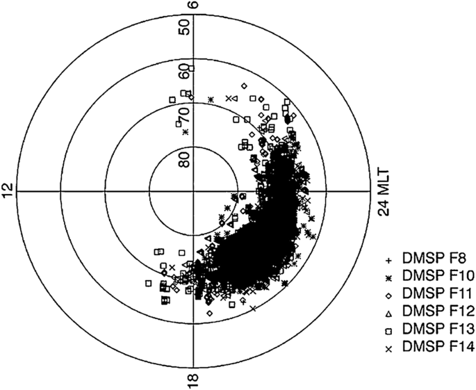

  

  Distribution of local time of LEO DMSP satellite anomalies (Anderson 2012)

Figures 7 and 8 show similar morphologies of the local time of anomalies, with distribution mostly within the dusk-to-midnight sector. Although this morphology varies depending on the case, both our study and Anderson (2012) showed good correlation between LEO anomalies and lower-energy electrons.

Conclusion

We investigated the proximate cause of anomalies on LEO satellites and found that around 60% of anomalies in this study were strongly related to lower-energy electron fluxes of 30–100 keV and to associated magnetic perturbations through Kp and Dst indices. The anomalies tended to follow three patterns: They occurred during the main phase of a magnetic storm (pattern 1), as incurred by ASCA (case #2; Fig. 4a); they coincided with the recovery phase of a storm (pattern 2), as shown in FUSE (1) (case #4; Fig. 4b), DART (Additional file 3: case #12), and Monitor-E (Additional file 4: case #13); or they were attributed to multiple storms prior to and after the anomaly day (pattern 3), such as that in Radarsat-1(1) (case #7; Fig. 4d), Terra (Additional file 5: case #3), Yohkoh (Additional file 1: case #5b), Radarsat-1(2) (Additional file 6: case #8), Landsat 7 (Additional file 7: case #9), ICESat (Additional file 8: case #10), and Midori (Additional file 9: case #11). We also noted that among these three patterns, the LEO anomalies were linked most often to pattern 3 (40%). For the remaining cases, such as FUSE (2) (Additional file 1: case #5a), Aqua (Additional file 10: case #6), and from case #14(Kirari) to case #19 (Orbcomm) (Additional files 2, 11, 12, 13, 14, and 15) in Table 4, the anomaly occurrences were weakly linked to the geophysical parameters used in this study. Nevertheless, the contribution of lower-energy electron fluxes and their associated geomagnetic disturbances have played a role in these cases. In particular, the anomaly on FUSE (2) (Additional file 1: case #5a) resembled the FUSE (1) (case #4; Fig. 4b) malfunction and might represent worsening of the initial damage to the FUSE satellite.

The determination of SLT using the LAN parameter resulted in small deviations between local time derived from SND data and that extracted from TLE data. The deviations were less than 2 min, as shown in Table 3. Although the LAN parameter changed over time, its oscillation per day was very small, resulting in discrepancies of minutes and seconds but not hours (Table 3, column 4). Because this parameter can represent the position of the satellite relative to the Sun, it is relevant for determining the mean SLT with respect to the Sun in association with energetic particle injection in the nightside magnetotail.

Figure 7 shows that the local times of LEO anomalies were scattered primarily within two sectors: pre-dusk and pre-midnight. Because we intended to relate the anomalies to the migration of low-energy electrons in the nightside of the magnetosphere, we inferred that the LEO anomalies in this study occurred predominantly in the dusk-to-dawn sector of MLT. This phenomenon was noted in 65% of the occurrences. During geomagnetic disturbances, energetic electrons accelerated in the magnetotail plasma sheet and drifted into the ring current. A large portion of these energetic electrons, which have complex motions, were lost, precipitated into the upper atmosphere, and immersed LEO satellites in electron fluxes. This was evident in the flux variation in lower-energy channels as a result of magnetic perturbations represented by the Kp and Dst indices.

Appendix

Variation of electron fluxes and Kp and Dst indices within selected intervals for other anomaly cases given in Table 4.

Table 4 LEO satellite anomalies during the period 2000–2008 including brief description of failure

References

Anderson PC (2012) Characteristics of spacecraft charging in low Earth orbit. J Geophys Res 117:A07308.https://doi.org/10.1029/2011JA016875
Anderson PC, Koons HC (1996) Spacecraft charging anomaly on a low-altitude satellite in an aurora. J Spacecraft Rockets 33(5):734–738. https://doi.org/10.2514/3.26828
Asikainen T, Mursula K (2008) Energetic electron flux behaviour at low L-shells and its relation to the South Atlantic Anomaly. J Atmos Terr Phys 70:532–538
Asikainen T, Mursula K (2013) Correcting the NOAA/MEPED energetic electron fluxes for detector efficiency and proton contamination. J Geophys Res 118(10):6500–6510. https://doi.org/10.1002/jgra.50584
Belov A, Dorman L, Iucci N, Kryakunova O, Ptitsyna N (2005) The relation of high- and low-orbit satellite anomalies to different geophysical parameters. In: Daglis IA (ed) Effects of space weather on technology infrastructure. Part of the NATO sciences series II: mathematic, physics and chemistry book series, vol 176. Kluwer Academic Publishers, Dordrecht, pp 147–163
Choi HS, Lee J, Cho KS, Kwak YS, Cho IH, Park YD, Kim YH, Baker DN, Reeves GD, Lee DK (2011) Analysis of GEO spacecraft anomalies: space weather relationship. Space Weather 9(6):1–12. https://doi.org/10.1029/2010SW000597
Evans DS, Greer MS (2004) Polar orbiting environmental satellite space environment monitor-2: instrument description and archive data documentation. NOAA technical memorandum OAR SEC 93. Available at ftp://satdat.ngdc.noaa.gov/sem/poes/docs/sem2_docs/2006/SEM2v2.0.pdf. Accessed 21 November 2017
Farthing WH, Brown JP, Bryant WC (1982) Differential spacecraft charging on the geostationary operational environmental satellites. NASA technical memorandum 83908. Available at https://ntrs.nasa.gov/archive/nasa/casi.ntrs.nasa.gov/19820018480.pdf. Accessed 7 November 2017
Fennell JF, Koons HC, Roeder L, Blake JB (2001) Spacecraft charging: observations and relationship to satellite anomalies. In: Harris RA (ed) Proceeding of the seventh international conference, ESTEC, Noordwijk, the Netherlands, 23–27 April 2001
Gonzales WD, Joselyn JA, Kamide Y, Kroehl HW, Rostoker G, Tsurutani BT, Vasyliunas VM (1994) What is geomagnetic storm? J Geophys Res 99(A4):5771–5792. https://doi.org/10.1029/93JA02867
Gubby R, Evans J (2002) Space environment effects and satellite design. J Atmos Terr Phys 64(16):1723–1733. https://doi.org/10.1016/S1364-6826(02)00122-0
Gussenhoven MS, Hardy DA, Rich F, Burke WJ, Yeh HC (1985) High-level spacecraft charging in the low-altitude polar auroral environment. J Geophys Res 90(A11):11009–11023. https://doi.org/10.1029/JA090iA11p11009
Hastings DE (1995) A review of plasma interactions with spacecraft in low Earth orbit. J Geophys Res 100(A8):14457–14483. https://doi.org/10.1029/94JA03358
Hastings D, Garret H (1996) Spacecraft environment interaction. Cambridge University Press, Cambridge
Iucci N, Dorman LI, Levitin AE, Belov AV, Eroshenko EA, Ptitsyna NG, Villoresi G, Chizhenkov GV, Gromova LI, Parisi M, Tyasto MI, Yanke VG (2006) Spacecraft operational anomalies and space weather impact hazards. Adv Space Res 37(1):184–190. https://doi.org/10.1016/j.asr.2005.03.028
Kichak RA (2011) Independent GLAS anomaly review board executive summary. Available at https://icesat.gsfc.nasa.gov/icesat/docs/IGARB.pdf. Accessed 25 July 2017
Koons HC, Mazur JE, Selesnick RS, Blake JB, Fennell JF, Roeder JL, Anderson PC (2000) The impact of the space environment on space systems. In: Proceedings of the 6th spacecraft charging conference, AFRL science center, 1 September 2000
Lai ST (2012) Fundamentals of spacecraft charging: spacecraft interactions with space plasmas. Princeton University Press, Princeton
Lam HL, Hruska J (1991) Magnetic signatures for satellite anomalies. J Spacecraft 28(1):93–99. https://doi.org/10.2514/3.26214
Lam MM, Horne RB, Meredith NP, Glauert SA, Griffin TM, Green JC (2010) Origin of energetic electron precipitation >30 keV into the atmosphere. J Geophys Res 115(A4):A00F08. https://doi.org/10.1029/2009JA014619
Lohmeyer W, Cahoy K, Baker DN (2012) Correlation of GEO communication satellite anomalies and space weather phenomena: improved satellite performance and risk mitigation. In: 30th AIAA international communications satellite system conference (ICSSC), Ottawa, Canada, 24–27 September 2012. https://doi.org/10.2514/6.2012-15083
NASA’s Goddard Space Flight Center (NASA GSFC)(2016) OMNIweb data documentation. https://omniweb.gsfc.nasa.gov/html/ow_data.html. Accessed 15 September 2016
NOAA’s National Center for Environmental Information (NOAA NCEI) (2017) POES space environment monitor data and documentation. http://satdat.ngdc.noaa.gov/sem/poes/data. Accessed 17 April 2017
O’Brien TP (2009) SEAS-GEO: a spacecraft environmental anomalies expert system for geosynchronous orbit. Space Weather 7(9):1. https://doi.org/10.1029/2009SW000473
Patil CG, Rajaram G, Prasad MYS (2008) Correlation of GSO satellite anomalies with space weather data. Acta Astronaut 63(1–4):458–470. https://doi.org/10.1016/j.actaastro.2007.12.050
Peck ED, Randall CE, Green JC, Rodriguez JV, Rodger CJ (2015) POES MEPED differential flux retrievals and electron channel contamination correction. J Geophys Res 120(6):4596–4612. https://doi.org/10.1002/2014JA020817
Pilipenko V, Yagova N, Romanova N, Allen J (2006) Statistical relationship between satellite anomalies at geostationary orbit and high-energy particles. Adv Space Res 37(6):1192–1205. https://doi.org/10.1016/j.asr.2005.03.152
Prolss GW (2004) Physics of the Earth’s space environment: an introduction. Springer, Berlin
Robertson B, Stoneking E (2003) Satellite GN&C anomaly trends. In: 2003 AAS guidance and control conference, American Astronautical Society guidance and control conference, Breckenridge, United States, 5–9 February 2003
Rodger CJ, Clilverd MA, Green JC, Lam MM (2010) Use of POES SEM-2 observations to examine radiation belt dynamics and energetic electron precipitation into the atmosphere. J Geophys Res. https://doi.org/10.1029/2008JA014023
Satellite News Digest (SND) (2017) Satellite outages and failures. https://www.sat-nd.com. Accessed 2 August 2017
SIA (2015) State of the satellite industry report – September 2015. Available at http://www.sia.org Accessed 22 Desember 2015
Space-Track (2015) Two-line element set database. https://www.space-track.org. Accessed 18 November 2015
Tadokoro H, Tsuchiya F, Miyoshi Y, Misawa H, Morioka A, Evans DS (2007) Electron flux enhancement in the inner radiation belt during moderate magnetic storms. Ann Geophys 25(6):1359–1364. https://doi.org/10.5194/angeo-25-1359-2007
Thomsen MF, Henderson MG, Jordanova VK (2013) Statistical properties of the surface-charging environment at geosynchronous orbit. Space Weather 11(5):237–244. https://doi.org/10.1002/swe.20049
Union of Concerned Scientists (UCS) (2015) UCS satellite database. https://www.ucsusa.org. Accessed 22 December 2015
Vallado DA, McClain WD (1997) Fundamentals of astrodynamics and applications. McGraw-Hill, New York
Vallado DA, Crawford P, Hujsak R, Kelso TS (2006) Revisiting Spacetrack report #3. In: AIAA/AAS astrodynamics specialist conference and exhibit, Keystone, Colorado, 21-24 August 2006. https://doi.org/10.2514/6.2006-6753
Vampola AL (1994) Analysis of environmentally induced spacecraft anomalies. J Spacecraft Rockets 31(2):154–159. https://doi.org/10.2514/3.26416
Welling DT (2010) The long-term effects of space weather on satellite operations. Ann Geophys 28(6):1361–1367. https://doi.org/10.5194/angeo-28-1361-2010
Wing S, Gkioulidou M, Johnson JR, Newell PT, Wang CP (2013) Auroral particle precipitation characterized by the substorm cycle. J Geophys Res 118(3):1022–1039. https://doi.org/10.1002/jgra.50160
Wu CC, Liou K, Lepping RP, Meng CI (2004) Identification of subtorms within storms. J Atmos Terr Phys 66(2):125–132. https://doi.org/10.1016/j.jastp.2003.09.012
Authors’ contributions
NA was involved in research of LEO satellite anomalies associated with space weather parameters and contributed to the manuscript and figure preparation. DH was responsible for space weather-related anomaly research and wrote the manuscript. TD prepared the analyses of satellite orbits, applied the SGP4 code used in this research, and assisted with the manuscript revision. HU and YM were involved in the spacecraft and plasma interaction research and provided comments and suggestions for the manuscript. All authors read and approved the final manuscript.
Authors’ information
Nizam Ahmad: The author works for Indonesian National Institute of Aeronautics and Space (LAPAN) in the field of spacecraft anomaly and celestial mechanics research. Currently, the author is taking a Ph.D. course in the Graduate School of System Informatics, Kobe University, Japan, and conducting research related to spacecraft and plasma interaction through the Electro-magnetic Spacecraft Environment Simulator (EMSES). The Ph.D. study program has been registered under sponsorship of the Ministry of Research and Technology, Secretariat of Project Management Office (PMO) Research and Innovation in Science and Technology Project (RISET-PRO) (REf.No.:7/RISET-Pro/SFS/I/2014). Dhani Herdiwijaya: Currently, the author serves as senior researcher and lecturer at the Institut Teknologi Bandung (ITB), Indonesia, in the field of astronomy, specifically in solar physics and space plasma. Thomas Djamaluddin: The author serves as chair of the Indonesian National Institute of Aeronautics and Space (LAPAN). The author also serves as professor in the field of astronomy and celestial mechanics. Hideyuki Usui: The author serves as professor in the Graduate School of System Informatics, Kobe University, Japan. The author has also conducted research in the field of space plasma including its interaction with spacecraft as well as wave–particle interactions in space plasmas. Yohei Miyake: The author serves as associate professor in the Graduate School of System Informatics, Kobe University, Japan (H. Usui’s research group) and has written and published many papers related to spacecraft and plasma interaction.
Acknowledgements
The authors would like to thank Kobe University, Institut Teknologi Bandung, and the Indonesian National Institute of Aeronautics and Space for providing facilities and other support for this research. The main author specifically thank the Ministry of Research and Technology under Secretariat of Project Management Office (PMO) Research and Innovation in Science and Technology Project (RISET-PRO) for supporting and facilitating activities during the Ph.D. study program. Also appreciated are the U.S. National Oceanic and Atmospheric Administration, U.S. National Aeronautics and Space Administration, and Space-Track, which provided much of the data used in this study. Special thanks are extended to Dr. Kelso, of Celestrak, for his instruction on applying SGP4 to local time calculations. In addition, David Eagle, of the MathWorks community, is appreciated for sharing the orbital and celestial mechanics codes. Finally, the authors express gratitude to the reviewers for providing helpful suggestions.
Competing interests
The authors declare that they have no competing interests.
Consent for publication
Not applicable.
Ethics approval and consent to participate
Funding
The submission of the manuscript was funded by Kobe University.
Publisher’s Note
Springer Nature remains neutral with regard to jurisdictional claims in published maps and institutional affiliations.
Author information
Authors and Affiliations
Corresponding author
Additional files
Additional file 1.
Variation of geophysical parameters around the anomaly day of FUSE (2) (case #5a) and Yohkoh (case #5b) satellites.
Additional file 2.
Variation of geophysical parameters around the anomaly day of Kirari satellite (case #14).
Additional file 3.
Variation of geophysical parameters around the anomaly day of DART satellite (case #12).
Additional file 4.
Variation of geophysical parameters around the anomaly day of Monitor-E satellite (case #13).
Additional file 5.
Variation of geophysical parameters around the anomaly day of Terra satellite (case #3).
Additional file 6.
Variation of geophysical parameters around the anomaly day of Radarsat 1(2) satellite (case #8).
Additional file 7.
Variation of geophysical parameters around the anomaly day of Landsat 7 satellite (case #9).
Additional file 8.
Variation of geophysical parameters around the anomaly day of ICEsat satellite (case #10).
Additional file 9.
Variation of geophysical parameters around the anomaly day of Midori satellite (case #11).
Additional file 10.
Variation of geophysical parameters around the anomaly day of Aqua satellite (case #6).
Additional file 11.
Variation of geophysical parameters around the anomaly day of KOMPASS 2 satellite (case #15).
Additional file 12.
Variation of geophysical parameters around the anomaly day of HST satellite (case #16).
Additional file 13.
Variation of geophysical parameters around the anomaly day of MetOp-A satellite (case #17).
Additional file 14.
Variation of geophysical parameters around the anomaly day of Orbview 3 satellite (case #18).
Additional file 15.
Variation of geophysical parameters around the anomaly day of Orbcomm satellite (case #19).