Relationship between topography, tropospheric wind, and frequency of mountain waves in the upper mesosphere over the Kanto area of Japan

Abstract

Imaging observations of OH airglow were performed at Meiji University, Japan (35.6° N, 139.5° E), from May 2018 to December 2019. Mountainous areas are located to the west of the imager, and westerly winds are dominant in the lower atmosphere throughout the year. Mountain waves (MWs) are generated and occasionally propagate to the upper atmosphere. However, only four likely MW events were identified, which are considerably fewer than expected. There are two possible reasons for the low incidence: (1) MWs do not propagate easily to the upper mesosphere due to background wind conditions, and/or (2) the frequency of MW excitation was low around the observation site. Former possibility is found not to be a main reason to explain the frequency by assuming typical wind profiles in troposphere and upper mesosphere over Japan. Thus, frequency and spatial distribution of orographic wavy clouds were investigated by analyzing images taken by the Himawari-8 geostationary meteorological satellite in 2018. The number of days when wavy clouds were detected in the troposphere around the observation site (Kanto area) was about a quarter of that around the Tohoku area. This result indicates that frequency of over-mountain flow which is thought to be a source of excitation of MWs is low in Kanto area. We also found that the angle between the horizontal wind direction in troposphere and the orientation of the mountain ridge is a good proxy for the occurrence of orographic wavy clouds, i.e., excitation of MWs. We applied this proxy to the topography around the world to investigate regions where MWs are likely to be excited frequently throughout the year to discuss the likelihood of "MW hotspots" at various spatial scale.

Graphical Abstract

Introduction

Atmospheric gravity waves (AGWs) propagate horizontally and vertically in the atmosphere. AGWs play an important role in the transport of energy and momentum from the excitation source to distant places. The most obvious sources of AGWs include topography, convection, wind shear, and jet/frontal systems, although other sources may also be important at certain sites or in association with specific large-scale dynamics (Fritts and Alexander 2003; Plougonven and Zhang 2014). AGWs induced by topography are referred to as mountain waves (MWs), and one of the most remarkable features of MWs is that they do not have an apparent phase speed if they are observed from the ground.

AGWs can propagate vertically in the atmosphere if there is no critical level or turning level on the ray path. If the apparent horizontal phase velocity (the horizontal phase velocity observed from the ground) of the AGW and the background horizontal wind velocity are equal, then this altitude is referred to as the critical level (Booker and Bretherton 1967). If there is a critical level in the vertical propagation path of the AGWs, then the waves cannot propagate above this altitude. Eventually, MWs are absorbed and dissipate into the background atmosphere at this altitude and transfer their momentum and energy to the background. AGWs are reflected at the altitude at which ${m}^{2}=0$ (where m is the vertical wave number), and this altitude is referred to as the turning level (Fritts and Alexander 2003). Tomikawa (2015) showed that AGWs with shorter horizontal wavelengths are more likely to be blocked from propagating vertically due to the turning level reflection. In addition, since the background atmospheric density decreases with altitude, the amplitude of the wave increases, and eventually the AGW breaks. In such cases, both momentum and energy are deposited into the background atmosphere. The momentum that is transferred from the lower to the middle atmospheres drives the circulation of the middle atmosphere.

When MWs propagate upward and reach a critical level, they form a weak wind layer near the mesopause region (Wang et al. 2006). Given that the excitation source of MWs is fixed on the ground, together with seasonal variations in background winds, MWs play an important role in affecting the rhythm of circulation in the middle atmosphere. Understanding the excitation and propagation processes of MWs is therefore important for quantifying global atmospheric circulation (Fritts and Alexander 2003).

Several observational studies of MWs have been conducted. For example, it has been shown that MWs are easily induced by the New Zealand landmass and the Antarctic Peninsula, both of which act as obstacles to winds in the lower atmosphere blowing over the Antarctic Ocean (Plougonven et al. 2008; Taylor et al. 2019). The MWs that are induced in these areas are frequently detected on the leeward side of the terrain (Espy et al. 2006; Ehard et al. 2017). It has also been reported that MWs generated by the Andes frequently propagate into the upper mesosphere (an altitude of approximately 85 km) (Smith 2009; Criddle et al. 2011; Hecht et al. 2018; Pautet et al. 2021). Smith et al. (2016) showed that MWs with long (60–120 km) or intermediate (20–60 km) horizontal wavelength contribute to carry momentum flux by analyzing aircraft observation data acquired during the Deep Propagating Gravity Wave Experiment (DEEPWAVE) campaign (Fritts et al. 2016). However, there are still numerous uncertainties in terms of the relationship between the excitation frequency, propagation process, or shape of the source mountain (Sandu et al. 2019). At present, general circulation models (GCMs) cannot adequately handle the effects of small-scale (< 100 km) AGWs, such as some MWs. Although a variety of methods have been proposed for parameterizing the effects of small AGWs in many models, more observations are required to improve the models (Yigit et al. 2009; Richter et al. 2010).

In this study, imaging observations of OH (7–3) airglow at the Kawasaki City campus of Meiji University, Japan (35.6° N, 139.5° E) were conducted from May 2018 to December 2019 (Fig. 1). The objective of the observations was to estimate the frequency of MWs that propagate from a mountainous region into the upper mesosphere over the observation site. The mountainous area located to the west of the observation site includes Mt. Fuji, which is the highest mountain in Japan. Since MWs are induced by topography, it is considered that the characteristics of MWs are affected by the underlying topographical features. The observation data were used to analyze the propagation frequency and the horizontal scale parameters of the MWs.

Fig. 1

Location of the observation site at Meiji University, Kawasaki, Japan (Geospatial Information Authority of Japan 2020)

In the latter part of this paper, the frequency of MW excitation from mountains with small horizontal scale (~ 80 km) is estimated. The Himawari-8 geostationary meteorological satellite (GMS-8) monitors the cloud distribution over an area around Japan with a high spatial horizontal resolution of 1 km (Bessho et al. 2016). When the atmosphere contains a sufficient amount of water vapor, wavy clouds are often generated near the mountainous area. These wavy clouds are often captured in GMS-8 RGB images. We estimated the excitation frequency of MWs over Japan by detecting the wavy clouds in GMS-8 RGB images acquired in 2018.

Details regarding the airglow observation instruments, observation settings, and methods for analyzing the airglow image data are described in section “Observations and analysis”. The results of the airglow imaging observations conducted at Meiji University from May 2018 to December 2019 are presented in section “Observation results”. In section “Discussion”, the occurrence of over-mountain flow in Japan and the frequency of the observed MWs are discussed based on an analysis of cloud images acquired by the GMS-8. A summary of our findings and conclusions is presented in section “Summary and conclusion”.

Observations and analysis

Instrumentation

In this study, OH airglow imaging observations were conducted at Meiji University, Kawasaki, Japan (35.6° N, 139.5° E) from May 2018 to December 2019. The objective of these observations was to detect MWs that were induced by a lower atmosphere, westerly wind blowing over the mountainous areas and Mt. Fuji located to the west of the observation site (Fig. 1).

A cooled CCD camera (Clara, Andor Technology Ltd., UK) was used for all observations. Table 1 and Fig. 2 show the main specifications and components of the camera, respectively. Specifically, the camera consists of a fish-eye lens (objective lens), a mechanical shutter, a collimator lens, an interference filter, a focusing lens, and the detector. The bandpass interference filter, which is 15 nm wide and is centered at 890 nm, is optimized to detect emissions from the Meinel OH (7–3) band in the near-infrared wavelength (Johnston and Broadfoot 1993). Figure 3 shows a transmittance profile of the interference filter with locations of the major rotational lines belonging to the Meinel OH (7–3) band. This wavelength region was selected because it is less contaminated by light pollution from surrounding urban areas. The collimator lens is set in front of the filter to suppress the effect of a wavelength shift in the bandpass filter which can arise depending on the angle of incident light to the filter. The imager was placed in a waterproofed box for field observations; specifically, the box was equipped with a thermostatically controlled heater and intake fan to ensure that the temperature and humidity inside the box remained between 5 and 25 °C, and less than 65%, respectively. A mechanical shutter behind the fish-eye lens prevents damage to the CCD due to direct sunlight. This shutter is controlled by a trigger signal sent from the camera.

Table 1 Specifications of the Clara CCD camera

Fig. 2

Optical components of the OH airglow imager

Fig. 3

Transparency characteristics of the interference filter. The wavelengths of the Q-branch and the P-branch in the OH (7–3) band are indicated by arrows above the image

Figure 4 shows the field of view (FOV) of the imager at a typical altitude for the OH layer (85 km) (Liu and Shepherd 2006). The effective FOV at this altitude has a radius of about 120 km from the observation site, the exposure time was 3 min, and the images were taken continuously from sunset to sunrise. To obtain airglow images with a high signal-to-noise ratio (SNR), 2 × 2 binning was performed on the CCD. The final image acquired by the imager measured of 696 pixels × 520 pixels. The dark frame used for the dark subtraction method described in section “Procedure for extracting MW signals from image data” was taken every night with the shutter closed at the start of observation. The imager was controlled by a PC installed in the box, and all of the acquired image data were saved in TIFF format.

Fig. 4

Geographical projection of an OH airglow image acquired at 2:53 JST on January 18, 2019. The image also shows the effective field of view at the altitude of the OH airglow layer (85 km). The red star indicates the location of the observation site

Definition of valid data

Airglow cannot be observed from the ground in cloudy weather conditions. In addition, data with moon light and the associated scattered light were excluded from the analysis because this source of light contamination is considerably stronger than the airglow emission. In this study, image data that satisfied the following two conditions were defined as valid data for further analysis:

• (1) Data were acquired on a clear night.

• (2) Data without the moon, the associated scattered light, and following stray light causing ghosting and/or flaring.

We visually checked the image data and judged its validity by focusing on the presence of stars. Figure 5a–c shows examples of valid and invalid data. When valid data were obtained continuously for several hours, the images were subjected to MW analysis using the method described in section “Procedure for extracting MW signals from image data”.

Fig. 5

a Example of a valid image. b and c invalid image data with the moon and clouds, respectively

Procedure for extracting MW signals from image data

The following analytical method was used to extract MW signals from airglow image data. Since the apparent horizontal phase speed of the MW is zero, the MW would appear to be almost stationary to an observer on the ground. In principle, the bright and dark patterns in an airglow image generated by the MWs would become clear by simply integrating the successive images. However, due to the van Rhijn effect, atmospheric extinction effects, and inhomogeneous sensitivity of the optics, simple integration does not enhance the MW signatures with horizontal wavelengths that have same order as the FOV (see Fig. 4). The procedure employed to remove these effects from the integrated airglow image data is described below.

First, the elevation and the azimuth angles corresponding to each pixel of an image are determined using star images (Fig. 6). A scheme to fit the local horizontal coordinate system to images was described in Suzuki et al. (2015). The azimuth angle, which is the angle from true north, increases counterclockwise in an image. As shown in Fig. 6, data captured at an elevation angle of < 30° cannot be used in the analysis due to FOV obstruction by ground artifacts; however, data captured at an elevation angle > 30° could be used for analysis in this study. Second, dark counts were removed by subtracting the dark frame. Third, point-like structures, such as bright stars, were attenuated by using a 5 pixel × 5 pixel median filter.

Fig. 6

Elevation and azimuth angles fitted to an airglow image. Red contour lines show elevation angles, and red dashed lines show azimuth angles. The right and top sides of the image indicate south and west, respectively. The azimuth is set to 0° northward and increases counterclockwise in an image

The valid data acquired continuously for 2 h, which correspond to 40 images, were averaged (we call this averaged data $\overline{{\varvec{I}} }$) (Fig. 7a). This process smooths the wave with non-zero horizontal phase speed. By this method, stationary AGWs with a horizontal scale smaller than the FOV (horizontal wavelength < 240 km) can be detected. Next, averaged counts at each elevation angle Φ were calculated from $\overline{{\varvec{I}} }$ to yield a count profile, $\overline{{\varvec{I}} }\left(\mathbf{\Phi }\right)$, which is a function of Φ. $\overline{{\varvec{I}} }\left(\mathbf{\Phi }\right)$ was calculated for the range of 30° < Φ < 90° for every 1 degree bin. The red line in Fig. 7b shows an example of $\overline{{\varvec{I}} }\left(\mathbf{\Phi }\right)$, and black plus symbols indicate $\overline{{\varvec{I}} }$. By subtracting the corresponding $\overline{{\varvec{I}} }\left(\mathbf{\Phi }\right)$ from the $\overline{{\varvec{I}} }$ for all pixels, azimuthally symmetrical effects, such as the van Rhijn effect and atmospheric extinction effects, were removed. Residual counts are axially unsymmetrical components in airglow image data. The amplitude of these residual components to $\overline{{\varvec{I}} }\left(\mathbf{\Phi }\right)$ is then calculated by $100 \times (\overline{{\varvec{I}} }-\overline{{\varvec{I}} }\left(\mathbf{\Phi }\right)$)/$\overline{{\varvec{I}} }\left(\mathbf{\Phi }\right)$ (%), as shown in Fig. 7c. We employed this procedure to identify and enhance the stationary and azimuthally unsymmetrical structures, i.e., possible MW signatures, in airglow image data. Image data were visually checked to judge whether a wavy structure was present in the residual counts (e.g., Fig. 7c).

Fig. 7

a Example image of “2 h-averaged count,” $\overline{{\varvec{I}} }$. Equivalent counts in each pixel are plotted in b as a function of the elevation angle with black symbols. The red line shown in b is the “elevation angle averaged count,” $\overline{{\varvec{I}} }\left(\mathbf{\Phi }\right)$. c Amplitude of the residual components ($\overline{{\varvec{I}} }-\overline{{\varvec{I}} }\left(\mathbf{\Phi }\right)$) to the $\overline{{\varvec{I}} }\left(\mathbf{\Phi }\right)$

Observation results

The total observation period was approximately 1 year and 8 months from May 2018 to December 2019. The observations were conducted automatically every night. The “observation time” simply refers to the time when the instruments were operated without system problems, and the “clear sky time” refers to the time over which the valid data were obtained (see section “Definition of valid data” for definition). The characteristics of these times over the entire observation period are summarized in Fig. 8. If valid data were acquired over two hours, then the airglow images were analyzed using the method described in section “Procedure for extracting MW signals from image data”. Table 2 shows the total number of observation days and nights with clear skies in every month.

Fig. 8

Summary of observation time and clear sky time

Table 2 Number of total observation days and nights with clear skies (> 2 h) in each month

We carefully analyzed all image data by applying the procedure outlined in section “Procedure for extracting MW signals from image data” and counted the number of events with a stationary wavy pattern (i.e., possible MW signatures). The results showed that stationary structures were detected only on four nights. Figure 9 shows examples of the stationary wave events projected onto geographic coordinates. The horizontal wavelength and the direction of the wavefront were roughly estimated from these images. Table 3 shows the horizontal parameters (the horizontal wavelength and the direction of the wavefront) and the duration of these four events. The observation of only four possible MW events is unexpectedly low considering that the observation site is located in a region that appears to be well suited for observing MWs (i.e., on the leeward side of mountains that would be expected to propagate MWs into the upper atmosphere).

Fig. 9

Possible MW events detected by the OH airglow imager during the observation period

Table 3 Horizontal parameters and duration of stationary waves detected in OH images

In section “Discussion”, we consider the reasons for the low number of possible MW events detected by the airglow observations. Specifically, we focused on the relationship between wind conditions in the lower atmosphere and features of the local orography to explain the results.

Discussion

The frequency of MW events revealed by the airglow imaging observations

We expected that numerous MWs would be induced by the mountainous area located to the west of the observation site, and that these MWs would propagate to the upper mesosphere. However, only four possible MW events were identified from the airglow observations over a period of approximately 1 year and 8 months (from May 2018 to December 2019).

We consider that there are two possible reasons for the low number of MWs observed in our study. First, although MWs may be induced by the mountainous area around Mt. Fuji, their vertical propagation may be impeded by the presence of a critical level and/or a turning level on the ray path. Second, fewer MWs are induced by the mountainous area around Mt. Fuji than in other mountainous areas.

We referred to the MERRA-2 (MERRA-2 tavg3_3d_asm_Nv: 3d, 3-Hourly, Time-Averaged, Model-Level, Assimilation, Assimilated Meteorological Fields V5.12.4) reanalysis data (Gelaro et al. 2017) to verify the wind fields on the days when the stationary structures were observed. The spatial resolution of the meteorological fields is 0.5° × 0.625° and the time interval is 3 h. We checked for the presence of a critical level in the horizontal wind profile in the direction perpendicular to the line of the wavefront for each event. This verification was conducted at altitudes ranging from 1,000 m to the upper limit of MERRA-2 (60 km) from the ground.

It was confirmed that the wind field during three events (2 June 2018, 1 February, and 15 December 2019) all had a critical level in this altitude range. This finding implies that these stationary structures were not a MW that was propagating from the mountains near the observation site. On the other hand, the wind profile during an event on 6 January 2019 had no critical level. The wind direction during the event was eastward from the lower layer to an altitude of 60 km. The horizontal wavelength of the event was about 50 km and the highest background wind speed during the event was about 50 m/s at an altitude of about 10 km. The intrinsic period of the wave at that altitude was about 1,000 s, so there was also no turning level. The wind condition allowed the vertical propagation of a MW. Figure 10 shows the horizontal wind speed component, U [m/s] projected in the direction of the wind at an altitude of 1,000 m (the red line shows the mean horizontal wind data from 21:00 to 27:00 JST on 6 January 2019). As shown in Fig. 8, January 2019 was the month with the longest period of clear skies in the entire observation period; the number of days that had clear skies for at least 2 h was 22 days. On these 22 days in January 2019, the nightly mean (18:00–27:00 JST) wind was projected in the wind direction at an altitude of 1,000 m from the ground (black lines in Fig. 10). Further, conditions on 13 of these 22 days were favorable for the vertical propagation of MW into the upper atmosphere (at least up to 60 km). Moreover, the wind profile on 6 January 2019 (red line) indicated the presence of highly suitable conditions during this period. Nevertheless, only one MW event was observed during this month.

Fig. 10

Horizontal wind speed component, U [m/s], projected in the wind direction at an altitude of 1,000 m from the ground. The red line shows the mean horizontal wind data from 21:00 to 27:00 JST on 6 January 2019. Black lines show the nightly mean (18:00–27:00 JST) wind profiles projected in the wind direction at an altitude of 1000 m from the ground on 22 clear nights in January 2019

In the same manner, wind fields were checked for the rest of the observation period. The results showed that favorable conditions for the vertical propagation of MWs occurred on 28 nights over the 20 months of the observation period. Like the event on 6 January 2019, a MW with a wave vector in the east–west direction and a wavelength of about 50 km may propagate vertically in winter. However, no other MW events were observed over the Kanto area in 2018 and 2019.

Based on the obtained findings, we focused on the second hypothesis, i.e., fewer MWs are induced by the mountainous area around Mt. Fuji than in other mountainous areas, to explain the unexpectedly low number of MW events in the airglow layer. We have verified the wind profile up to 60 km (the upper limit of MERRA-2). There is an unchecked region between z = 60 km and z = 85 km (height of the airglow layer). However, horizontal wind through this region in January is likely to be eastward according to long-term observations of mesospheric wind by using radars. The peak altitude and the amplitude of the zonal wind (mesospheric jet) in January are 70–75 km and + 40 m/s, respectively (Namboothiri et al. 1999). Zonal wind above the peak altitude gradually decreases to + 20 m/s till airglow height. Thus, the mean wind profile in January would increase in the eastward direction above 60 km. The typical amplitudes of diurnal and semidiurnal tides are in order of 5–15 m/s in January (Igarashi et al. 2002). Thus, zonal wind between the gap region should stay eastward in January if the typical wind field and amplitudes of tides are assumed. We therefore employed a simple proxy to explain the generation frequency of MWs in the mountainous area around Mt. Fuji in the next section.

Simple proxy to assess the frequency of MW excitation

When MWs are induced, wavy clouds, such as those shown in Fig. 11, are frequently generated on the leeward side of the mountainous area. Such clouds form when the winds in the lower atmosphere that are moving toward the orographic source contain sufficient water vapor to be saturated. These clouds have been observed frequently over Japan by the GMS-8 satellite (Bessho et al. 2016). However, if the atmosphere is dry, then there is a high possibility that wavy clouds will not appear, even if MWs are induced. Therefore, the absence of wavy clouds does not mean that MWs are not being induced. The formation of wavy clouds indicates that mountain-crossing airflow has occurred. Therefore, in this study, we assumed that MWs are induced whenever wavy clouds were formed on the leeward side of the mountains (e.g., see Fig. 11). In other words, we used the formation of wavy clouds as a proxy for the induction of MWs.

Fig. 11

Wavy clouds detected over the Tohoku area, Japan at 3:00 UT on June 22, 2018 by GMS-8

In this study, “wavy clouds” are defined as a set of three or more clouds oriented in parallel rows that are generated in the vicinity of mountainous areas. We examined the generation frequency and the spatial distribution of these wavy clouds over Japan by analyzing and visually checking color images acquired by GMS-8 in 2018. Specifically, we divided image data for Japan (3301 pixels × 2701 pixels) into smaller images (300 pixels × 300 pixels, i.e., 300 km × 300 km) and then checked if there were wavy clouds in each area. When wavy clouds were detected in a sub-image, we further subdivided the image into smaller sub-images (100 pixels × 100 pixels, i.e., 100 km × 100 km). The reason for subdividing the image into 100 km × 100 km sub-images was to investigate the generation and distribution of wavy clouds at a high spatial resolution. In addition, the direction of the wavefront, θ, and the distance between two adjacent clouds that make up a wavy cloud, i.e., the horizontal wavelength, λ, were calculated. Appendix 1 shows a detailed explanation of the procedure for deriving θ and λ.

Wavy clouds were typically stable and were continuously observed at the same location for several hours. Although the GMS-8 color image is acquired over 2.5 min, we analyzed the image data acquired every hour (taken at 9:00, 10:00, 11:00 … JST) during the day to simplify the analysis. When wavy clouds were detected in the same area in successive images, it was considered that the image represented the same event. The number of days when wavy clouds were observed was then counted for each sub-image (100 km × 100 km).

Frequency of wavy clouds over Japan

We analyzed GMS-8 color images acquired from January 2018 to December 2018 to identify wavy clouds over Japan. Figure 12a shows the occurrence frequency and spatial distribution of wavy clouds over Japan in this period. The color scale represents the number of days during which wavy clouds were observed. Wavy clouds were frequently observed over Hokkaido and the Tohoku region. Focusing on the Tohoku region, the area with the highest frequency was 79 days in 248 non-totally overcast days (Fig. 12b). In contrast, even over the highest area of the Kanto region, which is also within the FOV of our airglow imager, wavy clouds were detected only on 21 days in 239 non-totally overcast days. Furthermore, in most areas around the Kanto region, wavy clouds were detected only during approximately 10 days (Fig. 12c). These results showed that the occurrence frequency of wavy clouds differs markedly among regions, even though there are numerous mountainous areas throughout Japan.

Fig. 12

Number of days with wavy clouds in 2018 a over Japan and the surrounding area, b Tohoku region, and c Kanto region

The MERRA-2 data were used to calculate the wind velocity at an altitude of 1000 m from the ground at the center of each area and used as the background wind. Using this data set, we examined the angle between the wavefront direction and the background horizontal wind direction. Figure 13a shows the total occurrence frequency of the number of events with wavy clouds that were enumerated using this angle. The findings showed that more than 75% of wavy clouds had an angle ≥ 60°. The direction of the phase line of the wavy clouds was considered to reflect the orientation of the mountain ridgeline. Therefore, it was expected that MWs are frequently induced in regions where the angle between the direction of the background horizontal wind and the mountain ridgeline are ≥ 60°. A positive correlation was observed between the wavelength of the wavy clouds and the background wind speed (Fig. 13b). This relationship resembles the features of topographical wavy clouds reported by Fritz (1965). Although wavy clouds can be generated by a variety of mechanisms, i.e., not only by winds flowing over mountains but also by air masses colliding, frontal systems, convection, and wind shear, many of the wavy clouds detected in this study are likely to be caused by MWs.

Fig. 13

a Distribution of occurrence frequency of wavy cloud events enumerated based on the angle between the direction of the phase line of the wavy clouds and the background wind direction. b Relationship between the background wind speed at the altitude of 1000 m from the ground and the wavelength of wavy clouds detected over the Tohoku region

Relationship between topography and background wind in the lower atmosphere

The difference in the number of MWs generated over each region is considered to be the result of the interaction between topography and the synoptic horizontal wind field in the lower layers of the atmosphere. We examined the relationship between topographical features and the horizontal wind field by using geographical elevation data and meteorological reanalysis data. In this study, using the PNG Elevation Tile provided by the Geospatial Information Authority of Japan, the orientation of the mountain ridgeline (θ') was derived from the elevation data by the method shown in Appendix 2. The orientation of the mountain ridgeline is expressed as 0° ≤ $\theta ^{\prime}$≤ 180° (θ' = 0° represents that the mountain ridgeline faces east-west, and the angle increases counterclockwise).

We used MERRA-2 reanalysis data to examine the horizontal wind directions in the lower layer of the atmosphere. We adopted this wind field as a synoptic wind field. The wind velocity at an altitude of about 1000 m from the ground at the center of each elevation tile was calculated using these data. We defined the wind direction as being 0° when the wind blows eastward, with the angle increasing counterclockwise.

The acute angles between the horizontal wind directions and the direction of the mountain ridgelines (θ′) that were deduced using the above method were calculated for the entire world; we defined this angle as α. As mentioned in section “Frequency of wavy clouds over Japan”. 60° ≤ α ≤ 90° is considered to be favorable for inducing wavy clouds, i.e., over-mountain airflow, which is the primary source of MWs. Figure 14 shows the annual ratio, P, which satisfies the condition, 60° ≤ α ≤ 90° around Japan. Wind data at 10:30, 13:30, and 16:30 JST were used for this calculation because we wanted to compare the findings against the wave cloud occurrence frequency, which is derived from GMS-8 color images acquired during the day. The isolated data points surrounded by zero are omitted from this plot. The findings showed that these areas were highly consistent with the observed wavy cloud counts shown in Fig. 12. High values were clearly observed in the Tohoku and Hokkaido regions, and low numbers were clearly observed around the Kanto region.

Fig. 14

Annual occurrence of the condition satisfying 60° ≤ α ≤ 90°. The annual occurrence of 60° ≤ α ≤ 90° was calculated using 2920 wind values. The size of each cell was 40 km × 40 km. This value indicates the ratio for which favorable conditions occur for the induction of wavy clouds

The findings presented in Fig. 14 are consistent with the distribution of the occurrence frequency of wavy clouds. The simple proxy, $\alpha$, is considered to be well suited for predicting MW hotspots around the world. We estimated the global distribution of α in the same manner that was used to produce Fig. 14 and present the results in Fig. 15. The range of world elevation data used to derive α was between 70.6° S and 70.6° N and 180.0° W and 180.0° E. Importantly, all 3-h average wind data (8 wind values/day) are used in this calculation. Colored plots were observed in all of the major mountainous areas around the world (Fig. 15). For example, numerous colored plots were shown in the Andes and Antarctic Peninsula regions (surrounded by red circles in Fig. 15), which are well known sources of MWs. However, the findings showed that major mountainous areas are not “permanent” hot spots for wavy clouds. Indeed, the annual ratio of α in these regions being 60° ≤ α ≤ 90° is about 25–50%. In the high and mid-latitudes of the Northern Hemisphere, there are many locations where the ratio is > 25%, which is as high as that in the MW hotspots. In low-latitude regions, such as Mexico, northern Africa, southern India, and Southeast Asia, there are regions where the ratio is > 50%. Importantly, this plot merely shows the distribution of potential wavy cloud hot spots, i.e., the locations at which the active induction of MWs by over-mountain airflow may occur. Thus, it will be important to confirm the actual frequency of MWs being propagated into the upper atmosphere at these sites by further observations.

Fig. 15

Same as Fig. 14, except that the map shows the distribution of $\alpha$ at a global scale. The Andes Mountains and the Antarctic Peninsula are indicated by red circles

Comparison with model results

Sato et al. (2009) examined the origins of mesospheric gravity waves and the associated vertical flux in zonal momentum using a high-resolution global spectral climate model (KANTO model). Their model resolution was T213 (triangular truncation at wavenumber 213, which corresponds to about 60 km) in the horizontal direction and 300 m in the vertical direction. The horizontal wavelength resolved in the KANTO model is ≥ 188 km (Watanabe et al. 2008). Momentum flux is well suited for use as a diagnostic tool for estimating the effects of gravity waves because it is conserved, unless wave generation and/or dissipation occur (Eliassen and Palm 1961). Comparing their results with our Fig. 15 shows that the findings of the two studies are in good agreement in the Andes and the Antarctic Peninsula (red circles) where the effects of topographic gravity waves are dominant. On the other hand, Fig. 15 also shows that there are numerous small-scale (~ 80 km) hot spots in the mid-latitude regions of the Northern Hemisphere. The effect of such small areas on the atmospheric circulation is difficult to estimate in model calculations due to the limitations imposed by the spatial resolution of most models. However, we consider that the total contribution of these small areas is likely to be larger than that estimated in the study of Sato et al. (2009). Therefore, we expect that if the MWs that are induced in these small areas can propagate to the upper mesosphere, the total effects of those small excitation sources on circulation in the middle atmosphere are not negligible. In future work, we will investigate the propagation process of MW from small terrains and its impact on the upper atmosphere.

It is therefore considered necessary to conduct observations in order to verify how many MWs excited by such small areas can propagate to the upper mesosphere.

Summary and conclusion

Imaging observations of OH airglow was performed at Meiji University, Japan (35.6° N, 139.5° E) from May 2018 to Dec 2019 to reveal the occurrence frequency of MWs induced by the mountainous areas around Mt. Fuji that are located to the west of the imager. Careful analysis was applied to identify large stationary structures in the airglow images. However, the detection frequency of MWs in our observations (4 events/1 year and 8 months) was surprisingly low. In particular, the number of MW events observed in Jan 2019 was unexpectedly low, even if the frequency of clear days and background wind conditions are considered. To clarify this discrepancy, we examined the relationship between topography and horizontal wind fields using geographical elevation data and a model of meteorological fields.

First, we examined the occurrence frequency of wavy clouds that formed in the lower atmosphere around and over Japan by analyzing color image data obtained by the GMS-8 satellite. The results showed that wavy clouds formed in the leeward sides of mountain ridges and that the occurrence frequency of these clouds was high in northern regions of Japan and low in southern regions (including our observation site). Since this difference was considered to reflect the occurrence of over-mountain flow, which is a prerequisite for MW induction in mountainous areas, we then attempted to elucidate the underlying reasons for this spatial disparity. As a result, we developed a simple index, α, which is the angle between the orientation of mountain ridgeline and the background wind. This index can be used as a measure of the occurrence frequency of MW in each region. In addition, the index was confirmed to be a good proxy for explaining the occurrence frequency of wavy clouds. Since the condition α > 60° was found to be favorable for the induction of wavy clouds near mountainous areas, we mapped the global distribution of α. The results showed that areas where α > 60° were highly consistent with areas with high momentum flux to the upper atmosphere, as suggested by both previous observations and the GCM. In addition, it was found that there are numerous small areas that satisfy the condition α > 60° for more than a season at high and mid-latitudes in the Northern Hemisphere. Even though the size of these areas was small, the combined effect of the waves generated in each of these small areas may affect circulation in the middle atmosphere. It is therefore considered necessary to verify whether or not the MWs induced in these small areas can propagate to the middle atmosphere.

As a next step, we are planning to expand the OH airglow imaging observations to the Tohoku region and/or Hokkaido where the occurrence frequencies of MWs is expected to be higher. Performing such observations will allow us to clarify the effects of small-scale topography on circulation in the middle atmosphere.

Appendix

Appendix 1: Procedure for deriving the wavelength and wavefront direction of wavy clouds from GMS-8 image.

The wavelength and wavefront direction of the wavy clouds are derived from the GMS-8 image using steps (i) to (iv) below.

• (i) Divide image data for Japan (3301 pixels × 2701 pixels) into smaller images (300 pixels × 300 pixels, i.e., 300 km × 300 km) and check if there are wavy clouds in this area. If wavy clouds exist in a sub-image, further subdivide the image (100 pixels × 100 pixels, i.e., 100 km × 100 km) (Fig. 

  Fig. 16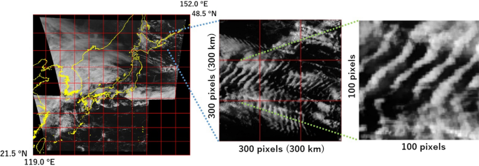

  

  Subdivision of the original GMS-8 image into sub-images to isolate wavy clouds for deriving wavelength and wavefront

  16) and move to the next step.

• (ii) Select two adjacent rows of clouds form a wavy cloud in a 100 pixel × 100 pixel image. Mark two points on the centerline of each cloud and acquire the position of each point on the image (Fig. 

  Fig. 17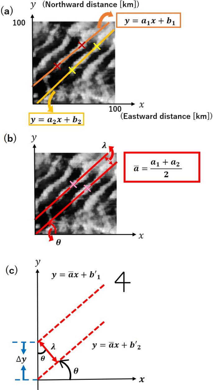

  

  a and b The method for calculating the wavelength, λ, and the wavefront, θ, of wavy clouds; c definition of the wavy cloud wavelength, λ, and the wavefront, θ

  17a). The positive values of the (x, y) coordinates in Fig. 17 corresponds to the (east, north) directions, respectively.

• (iii) The equations for the two straight lines are derived from the position acquired in ii). The gradients of each line are defined as ${a}_{1} \text{ and } {a}_{2}$, and the mean value, $\overline{a }$, of ${a}_{1} \text{ and } {a}_{2}$ is defined as the mean gradient of the two lines (Fig. 17b).

• (iv) The equations of the two straight lines with gradients $\overline{a }$ passing through the midpoint of the two points are derived for each cloud selected in (iii). The midpoints are point ${M}_{1}$ and point ${M}_{2}$ in Fig. 17b. Let the coordinates of point ${M}_{1}$ and point ${M}_{2}$ be $\left({x}_{1}, {y}_{1}\right)$ and $\left({x}_{2}, {y}_{2}\right)$, respectively. The Y-axis intercept, ${{b}^{^{\prime}}}_{1}$, for the equation is calculated by $b^{\prime}_{1} = y_{1} - \overline{a}x_{1}$. ${{b}^{^{\prime}}}_{2}$ is calculated in a similar manner. The distance between two cloud rows, i.e., the wavelength, $\lambda$, and the direction of the wavefront, θ, are obtained as shown in Fig. 17c. The difference between the Y-axis intercepts ${{b}^{\prime}}_{1}$ and ${{b}^{\prime}}_{2}$ of the two straight lines is defined as $\Delta y$, and λ is calculated by $\Delta y\text{cos}\theta$. We assumed θ to be 0° in the eastward direction and that it increases counterclockwise.

Appendix 2: Details of elevation data

First, we derived the elevation data by using PNG Elevation Tile provided by the Geospatial Information Authority of Japan (Fig. 

Fig. 18

Method for estimating elevation data. a “Elevation tile” provided by the Geospatial Information Authority of Japan, b elevation data calculated from the “elevation tile,” c mountain ridgeline extracted from b using the method of Iwahashi (1994), d enlarged view of the yellow inset in c and definition of the direction of the mountain ridgeline θʹ

18a) (Nishioka and Nagatsu, 2015). The elevation value for each pixel is calculated from the pixel value using Eqs. (1) and (2) as follows:

$$X = 2^{{16}} R + 2^{8} G + B$$

(1)

$$\left\{ \begin{gathered} H = Xh_{{{\text{res}}}} \left( {X < 2^{23} } \right) \hfill \\ H = 0 \left( {X = 2^{23} } \right) \hfill \\ H = \left( {X - 2^{24} } \right)h_{{{\text{res}}}} \left( {X > 2^{23} } \right) \hfill \\ \end{gathered} \right.,$$

(2)

where R, G, and B are the color components of the pixel value of the elevation tile, ${h}_{\text{res}}$ (= 0.01 m) is the elevation resolution, and H is the elevation value. Figure 18b shows the elevation converted from Fig. 18a. Then, mountain ridgelines were extracted from each tile using a median filter as described by Iwahashi (1994) to deduce the topographic features. The median filter is applied to the elevation data, and this result is defined as M. The position where $H\left(x, y\right)$ is larger than the median $M\left(x, y\right)$ of the 3 × 3 surrounding pixels is the mountain ridge $(\left(x, y\right)$ are the pixel coordinates of the image). Figure 18c shows the mountain ridgelines deduced from Fig. 18b. After smoothing fine structures less than 40 km, the elevation map of the extracted ridgelines was divided into squares of 40 km × 40 km, referred to here as “square blocks.” If a mountain ridgeline exists in a square block, then the orientation of the mountain ridgeline, $\theta ^{\prime}$, was calculated as follows. Rotate the image counterclockwise in 1° increments from 0 to 180° and calculate the standard deviation of elevation values vertically in the square block, and then add the horizontal direction obtained for each 1° increment. Then, find the rotation angle (RA) that minimizes that value. When the RA of the image is ≤ 90°, the orientation of the mountain ridgeline, $\theta ^{\prime}$, can be calculated as $\theta ^{\prime}$ = 90 – RA, and when RA is > 90°, $\theta ^{\prime}$ = 270 – RA. The orientation of the mountain ridgeline is expressed as 0° ≤ $\theta ^{\prime}$≤ 180° (Fig. 18d).

References

Bessho K, Date K, Hayashi M, Ikeda A, Imai T, Inoue H, Kumagai Y, Miyakawa T, Murata H, Ohno T, Okuyama A, Oyama R, Sasaki Y, Shimazu Y, Shimoji K, Sumida Y, Suzuki M, Taniguchi H, Tsuchiyama H, Uesawa D, Yokota H, Yoshida R (2016) An introduction to Himawari-8/9—Japan’s new-generation geostationary meteorological satellites. J Meteorol Soc Jpn 94:151–183. https://doi.org/10.2151/jmsj.2016-009
Booker JR, Bretherton FP (1967) The critical layer for internal gravity waves in a shear flow. J Fluid Mech 27:513–539
Criddle NR, Taylor M, Pautet P-D, Zhao Y (2011) Seasonal Variability and dynamics of mesospheric gravity waves over the Andes. 2011 Joint CEDAR-GEM Workshop. Graduate Student Posters. Paper 29
Ehard B, Kaifler B, Dornbrack A, Preusse P, Eckermann DS, Bramberger M, Gisinger S, Kaifler N, Liley B, Wagner J, Rapp M (2017) Horizontal propagation of large-amplitude mountain waves into the polar night jet. J Geophys Res 122:1423–1436
Eliassen A, Palm E (1961) On the transfer of energy in stationary mountain waves. Geofys Publ 22:1–23
Espy PJ, Hibbins RE, Swenson GR, Tang J, Taylor MJ, Riggin DM, Fritts DC (2006) Regional variations of mesospheric gravity-wave momentum flux over Antarctica. Ann Geophys 24:81–88
Fritts DC, Alexander MJ (2003) Gravity wave dynamics and effects in the middle atmosphere. Rev Geophys 41(1):1003. https://doi.org/10.1029/2001RG000106
Fritts DC, Smith RB, Taylor MJ, Doyle JD, Eckermann SD, Dörnbrack A, Rapp M, Williams BP, Pautet PD, Bossert K, Criddle NR (2016) The Deep Propagating Gravity Wave Experiment (DEEPWAVE): An airborne and ground-based exploration of gravity wave propagation and effects from their sources throughout the lower and middle atmosphere. Bull Am Meteor Soc 97:425–453. https://doi.org/10.1175/BAMS-D-14-00269.1
Fritz S (1965) The significance of mountain lee waves as seen from satellite pictures. J Appl Meteor 4:31–37
Gelaro R, McCarty W, Suárez MJ, Todling R, Molod A, Takacs L, Randles CA, Darmenov A, Bosilovich MG, Reichle R, Wargan K, Coy L, Cullather R, Draper C, Akella S, Buchard V, Conaty A, da Silva AM, Gu W, Kim G-K, Koster R, Lucchesi R, Merkova D, Nielsen JE, Partyka G, Pawson S, Putman W, Rienecker M, Schubert SD, Sienkiewicz M, Zhao B (2017) The modern-era retrospective analysis for research and applications, version 2 (MERRA-2). J Clim 30(14):5419–5454
Geospatial Information Authority of Japan (2020) https://www.gsi.go.jp/. Accessed 8th Feb 2020.
Global Modeling and Assimilation Office (GMAO) (2015) MERRA-2 tavg3_3d_asm_Nv:3d,3-Hourly,Time-Averaged,Model-Level,Assimilation,Assimilated Meteorological Fields V5.12.4, Greenbelt, MD, USA, Goddard Earth Sciences Data and Information Services Center (GES DISC). Accessed 8th Feb 2020, 10.5067/SUOQESM06LPK
Hecht JH, Fritts DC, Wang L, Gelinas LJ, Rudy RJ, Walterscheid RL, Franke SJ (2018) Observation of the breakdown of mountain waves over the Andes Lidar Observatory at Cerro Pachon on 8/9 July 2012. J Geophys Res 123:276–299
Igarashi K, Namboothiri SP, Kishore P (2002) Tidal structure and variability in the mesosphere and lower thermosphere over Yamagawa and Wakkanai. J Atmos Solar Terr Phys 64(8–11):1037–1053
Iwahashi J (1994) Development of landform classification using digital elevation model. Annuals Disas Prev Res Inst, Kyoto Univ, No. 37 B-1
Johnston JE, Broadfoot AL (1993) Midlatitude observations of the night airglow: implications to quenching near the mesopause. J Geophys Res 98:593–621
Liu G, Shepherd GG (2006) An empirical model for the altitude of the OH nightglow emission. Geophys Res Lett 33:9
Namboothiri SP, Tsuda T, Nakamura T (1999) Interannual variability of mesospheric mean winds observed with the MU radar. J Atmos Solar Terr Phys 61(15):1111–1122
NICT/Himawari-8 real-time web (2020) Himawari-8 real-time web. http://himawari8.nict.go.jp/. Accessed 8 Feb 2020.
Nishioka Y, Nagatsu J (2015) PNG elevation tile: design and implementation of the elevation file format for web use. Geoinformatics 26:155–163
Pautet P-D, Taylor MJ, Fritts DC, Janches D, Kaifler N, Drnbrack A, Hormaechea JL (2021) Mesospheric mountain wave activity in the lee of the Southern Andes. J Geophys Res. https://doi.org/10.1029/2020JD033268
Plougonven R, Hertzog A, Teitelbaum H (2008) Observations and simulations of a large-amplitude mountain wave breaking over the Antarctic Peninsula. J Geophys Res 113:D16113. https://doi.org/10.1029/2007JD009739
Plougonven R, Zhang F (2014) Internal gravity waves from atmospheric jets and fronts. Rev Geophys 52:33–76. https://doi.org/10.1002/2012RG000419
Richter JH, Sassi F, Garcia RR (2010) Toward a physically based gravity wave source parameterization in a general circulation model. J Atmos Sci 67(1):136–156
Sandu I, van Niekerk A, Shepherd TG et al (2019) Impacts of orography on large-scale atmospheric circulation. Npj Clim Atmos Sci 2:10. https://doi.org/10.1038/s41612-019-0065-9
Sato K, Watanabe S, Kawatani Y, Tomikawa Y, Miyazaki K, Takahashi M (2009) On the origins of mesospheric gravity waves. Geophys Res Lett 36:L19801. https://doi.org/10.1029/2009GL039908
Smith S, Baumgardner J, Mendillo M (2009) Evidence of mesospheric gravity-waves generated by orographic forcing in the troposphere. Geophys Res Lett 36:L08807. https://doi.org/10.1029/2008GL036936
Smith RB, Nugent AD, Kruse CG, Fritts DC, Doyle JD, Eckermann SD, Taylor MJ, Dörnbrack A, Uddstrom M, Cooper W, Romashkin P, Jensen J, Beaton S (2016) Stratospheric gravity wave fluxes and scales during DEEPWAVE. J Atmos Sci 73(7):2851–2869
Suzuki H, Chino H, Sano Y, Kadokura A, Ejiri MK, Taguchi M (2015) Imagingbased observations of low-latitude auroras during 2001–2004 at Nayoro, Japan. Earth Planets Space 67(1):1–11. https://doi.org/10.1186/s40623-015-0278-z
Wang L, Fritts DC, Williams BP, Goldberg RA, Schmidlin FJ, Blum U (2006) Gravity waves in the middle atmosphere during the MaCWAVE winter campaign: evidence of mountain wave critical level encounters. Annales Geophysicae 24(4):1209-1226. https://doi.org/10.5194/angeo-24-1209-2006
Watanabe S, Kawatani Y, Tomikawa Y, Miyazaki K, Takahashi M, Sato K (2008) General aspects of a T213L256 middle atmosphere general circulation model. J Geophysical Res. https://doi.org/10.1029/2008JD010026
Taylor MJ, Pautet PD, Fritts DC, Kaifler B, Smith SM, Zhao Y, Criddle NR, McLaughlin P, Pendleton WR Jr, McCarthy MP, Hernandez G (2019) Large-amplitude mountain waves in the mesosphere observed on 21 June 2014 during DEEPWAVE: 1. Wave development, scales, momentum fluxes, and environmental sensitivity. J Geophys Res 124:10364–10384. https://doi.org/10.1029/2019JD030932
Tomikawa Y (2015) Gravity wave transmission diagram. Ann Geophys 33:1479–1484. https://doi.org/10.5194/angeo-33-1479-2015
Yigit E, Medvedev AS, Aylward AD, Hartogh P, Harris MJ (2009) Modeling the effects of gravity wave momentum deposition on the general circulation above the turbopause. J Geophys Res 114:D07101. https://doi.org/10.1029/2008JD011132
Acknowledgements
Wind data used in this study were obtained from the Global Modeling and Assimilation Office (GMAO) (2015), MERRA-2 tavg3_3d_asm_Nv: 3d, 3-Hourly, Time-Averaged, Model-Level, Assimilation, Assimilated Meteorological Fields V5.12.4, Greenbelt, MD, USA, Goddard Earth Sciences Data and Information Services Center (GES DISC), and can be accessed at 1**0.5067/SUOQESM06LPK. RGB image data taken by Himawari-8 meteorological satellite were provided by Science Cloud operated by National Institute of Information and Communications Technology (NICT). Elevation tiles were provided by the Geospatial Information Authority of Japan.
Funding
This work was supported by a Research Project Grant (B) from the Institute of Science and Technology at Meiji University. This study was supported by National Institute of Polar Research (NIPR) through General Collaboration Project no. 30–8.
Author information
Authors and Affiliations
Contributions
SI operated OH airglow imager at Ikuta on site, managed data analysis, and wrote the first draft of the manuscript. MO designed and installed the OH airglow imager. SI, MO, and HS (corresponding author) discussed the analytical methods of the OH airglow image data. SI, HS, and YT discussed the methods used for estimating the mountain wave hotspots. All the authors contributed improving the manuscript. All the authors have read and approved the final manuscript.
Corresponding author
Ethics declarations
Ethics approval and consent to participate
Not applicable.
Consent for publication
Competing interests
The authors have no competing interests.
Additional information
Publisher's Note
Springer Nature remains neutral with regard to jurisdictional claims in published maps and institutional affiliations.