Earthquake forecast models for inland Japan based on the G-R law and the modified G-R law

Abstract

The frequency-magnitude distribution expressed by the Gutenberg-Richter (G-R) law is the basis of a simple method to forecast earthquakes. The frequency-magnitude distribution is sometimes approximated by the modified G-R law, which imposes a maximum magnitude. In this study we tested three earthquake forecast models: Cbv (the Constant b-value model) based on only the G-R law with a spatially constant b-value, Vbv (the Variable b-value model) based on only the G-R law with regionally variable b-values, and MGR (the Modified G-R model) based on the modified G-R or G-R law (chosen according to Akaike Information Criterion) with regionally variable b-values. We also incorporated aftershock decay and minimum limits of expected seismicity in these models. Comparing the results of retrospective forecasts by the three models, we found that MGR was almost always better than Vbv; Cbv was better than Vbv for short-term (one year) forecasts; little difference between MGR and Cbv for short-term forecasts; and MGR and Vbv tended to be better than Cbv for long-term (three years or longer) forecasts. We propose the use of MGR in the earthquake forecast testing experiment by the Collaboratory for the Study of Earthquake Predictability for Japan.

1. Introduction

An earthquake forecast testing experiment was started by the Collaboratory for the Study of Earthquake Predictability (CSEP) for Japan on November 1, 2009 (Nanjo et al., 2009). The main purposes of the experiment are to elicit the submission of statistical and physics-based models, to evaluate the performance of these earthquake forecast models, and to better understand the physics and statistics of earthquake occurrence. The target of the forecasts is to predict a seismicity rate (number of earthquakes in a predefined time window) for each magnitude bin at each predefined grid node within a predefined testing region.

The Gutenberg-Richter (G-R) law (Gutenberg and Richter, 1944) is the basis of a simple method to predict earthquakes (e.g., Earthquake Research Committee, 2006; Wiemer and Schorlemmer, 2007). The Earthquake Research Committee (2006), for example, estimated nationwide occurrence probabilities for earthquakes in Japan whose location cannot be predefined. They used the G-R law with a spatiotemporally constant b-value, which we call the Cbv (constant b-value) model here. However, because the b-value varies spatially (e.g., Wiemer and Wyss, 1997; Hirose et al., 2002a, b; Schorlemmer et al., 2005), we made an earthquake forecast model using b-values estimated for each region to capture the regionality of seis-micity, which we call the Vbv (variable b-value) model. The frequency-magnitude distribution is also sometimes approximated by the modified G-R law of Utsu (1974), which imposes a maximum magnitude and assumes that no earthquakes larger than that magnitude occur. Accordingly, we also made a model that uses the modified G-R law for regions where it fits the data better than the original G-R law, which we call the MGR (modified G-R) model.

This paper reports the results of comparison of retrospective forecasts made using the MGR, Vbv, and Cbv models.

2. The G-R and Modified G-R Laws for Frequency-Magnitude Distributions

2.1 The G-R law

The general property of the size distribution of earthquakes, that large earthquakes occur in small numbers and small earthquakes occur in large numbers, is well known. When the number of earthquakes with magnitudes from M to M + dM in a given region and a given period is defined as n(M)d M, their size distribution is approximated by the G-R law (Gutenberg and Richter, 1944) given by

(1)

where a and b are constants. Furthermore, cumulative frequency-magnitude distribution is given by

(1-2)

where N(M) is the number of earthquakes with greater or equal to M, and A is a constant expressed as A = a − log(b ln 10). The b-value, which indicates the slope of the linear curve in the frequency-magnitude distribution, is an especially important parameter. Many researchers report that b-value varies spatiotemporally (e.g., Suyehiro, 1966; Anderson et al., 1980; Wyss, 1990; Wiemer and Benoit, 1996; Wiemer and McNutt, 1997; Wiemer and Wyss, 1997; Murru et al., 1999; öncel and Wyss, 2000; Wyss et al., 2000; Gerstenberger et al., 2001; Hirose et al., 2002a, b; Schorlemmer et al., 2005), and the results of laboratory experiments by Scholz (1968) are often quoted to explain the spatiotemporal variation of b-values. Scholz (1968) conducted a rock fracturing experiment and showed that b-values decrease with an increase of the shear stress acting on a medium. Schorlemmer et al. (2005) also suggested the dependency of b-values on stress by showing the relationship of b-values and the type of focal mechanisms. All of these results support the spatial variation of b-values.

2.2 The modified G-R law

It is commonly found that a frequency-magnitude distribution is a convex-upward curve rather than a straight line (e.g., Utsu, 1974) and departs from the G-R law. That is, the number of larger or smaller earthquakes is fewer than expected from the G-R law. This sometimes happens when the catalog is incomplete because of magnitude saturation for large earthquakes or nondetection of small earthquakes.

However, a frequency-magnitude distribution can depart greatly from the G-R law even if the catalog is perfect (e.g., Utsu, 1974; Umino and Sacks, 1993). Umino and Sacks (1993) researched frequency-magnitude distributions of earthquakes in the crust and in the upper plane of the double seismic zone in the Pacific slab beneath northeast Japan, using the Tohoku University and JMA catalogs with aftershocks removed. They found that both frequency-magnitude distributions departed from the G-R law, to a slight degree for earthquakes in the crust and to a greater degree for those in the slab. They confirmed that the catalogs were complete for M ≥ 2.0 in the crust and M ≥ 2.1 in the upper plane in the slab by the method of Rydelek and Sacks (1989). Furthermore, they found no difference between frequency-magnitude distributions based on seismic wave duration magnitudes and amplitude magnitudes. Therefore, they suggested that this result is robust.

Utsu (1974) proposed a modification of the magnitude distribution, employing an upper limit to model convex-upward curves:

(2-1)

(2-2)

where a, b, and c are constants, and c represents an upper magnitude limit. This frequency-magnitude distribution approaches zero asymptotically as M approaches c. Constants a and b in Eq. (2-1) cannot be treated as equivalents of those in Eq. (1), although Eq. (2-1) adds only the logarithmic function of c- M to Eq. (1). The b-valueof theG-Rlaw indicates the inclination of the frequency-magnitude distribution whereas the inclination in Utsu’s modified G-R law is the function of b, c, and M. The a-value of the G-R law indicates the number of earthquakes of M = 0, but this is not necessarily true in the modified G-R law. To avoid confusion, in this paper we rewrite a, b, and c in Eqs. (2) as a _m , b _m , and c _m , respectively:

(3-1)

(3-2)

Furthermore, cumulative frequency-magnitude distribution is given by

(3-3)

(3-4)

(3-5)

It is obvious from Eqs. (3-2) and (3-4) that earthquakes with M ≥ c _m are not expected to occur by definition in the modified G-R law. However, there is a possibility that earthquakes with M ≥ c _m might occur in the real activity during the predicting period, especially when the modeling period is not long enough to include a large earthquake or the predicting period is very long. Therefore, we introduced a minimum limit of seismicity rate to cover the disadvantage of using the modified G-R law, which is discussed in Section 4.2.

2.3 Parameter estimation

We applied the maximum likelihood estimation method (Aki, 1965; Utsu, 1974) to estimate the b-value of the G-R law and the b _m - and c _m -values of the modified G-R law. However, as the parameters of the modified G-R law, unlike the G-R law, cannot be obtained analytically, we estimated them numerically using the Newton method (Mabuchi et al., 2002). The MGR model compares values of the Akaike Information Criterion or AIC (Akaike, 1974) calculated by applying the G-R and modified G-R laws to observed frequency-magnitude distributions for each region, adopting the law that yields the smaller AIC for each region, unless the difference in AIC was less than 1, in which case we used the G-R law (see Section 4.1).

3. Data and Target Earthquakes

We used the Japan Meteorological Agency (JMA) unified hypocenter catalog and selected inland earthquakes with depths of 30 km or less, then divided this data base into two groups, of which one was used for modeling and the other for testing.

As for data for modeling, in consideration of the de-tectability of earthquakes at different times in the past (K. Z. Nanjo, private communication), we selected earthquakes of M ≥ 5.0, M ≥ 4.0, M ≥ 3.0, and M ≥ 2.0 for the periods 1965–2007, 1980–2007, 1990–2007, and 2000–2007, respectively. To investigate the stability of the models, we prepared virtual catalogs of eight different time spans, extrapolating the number of events in each magnitude bin from the shorter record periods. The virtual catalogs cover periods of 36, 37,…, 43 years, corresponding to 1965–2000, 1965–2001, …, 1965–2007, respectively. For the 43-year catalog (1965–2007), for example, the numbers of earthquakes with M ≥ 5.0, M ≥ 4.0, M ≥ 3.0, and M ≥ 2.0 were multiplied by 43/43 (= 1), 43/28, 43/18, and 43/8, respectively, according to the number of years in their respective periods (43, 28, 18, and 8 years) of record (Fig. 1).

Fig. 1.

Frequency-magnitude distribution of data used to make models. Crosses denote the number of events per magnitude bin. Data periods vary depending on magnitude ranges: 1965–2007 for M ≥ 5.0, 1980–2007 for M ≥ 4.0, 1990–2007 for M ≥ 3.0, and 2000–2007 for M ≥ 2.0. Open circles denote the number of events in each magnitude bin after adjustment based on the length of data periods. Solid circles are cumulative number of events shown by open circles. Solid line represents the approximate cumulative distribution by the G-R law with A = 6.81, b = 0.87.

As for data for testing, we defined target earthquakes as those that were with depth ≥ 30 km and 5.0 ≥ M ≥ 9.0 occurring during the testing period just after the modeling period. Testing period lengths were set at one, three, five, and seven years.

4. Construction of the Modified G-R Earthquake Forecast Model

4.1 Procedure for calculating model parameters

• Step 1. We set 5483 grids with a spacing of 0.1° in latitude and longitude over Japan and selected earthquakes occurring within a region with a radius of 20 km from each grid (Fig. 2). A circular area with a radius of 20 km is almost equal to the area of the source region S (km²) of an M 7.0 event given by an empirical relation log S = 1.02M − 4.0 (Utsu and Seki, 1955).

  Fig. 2.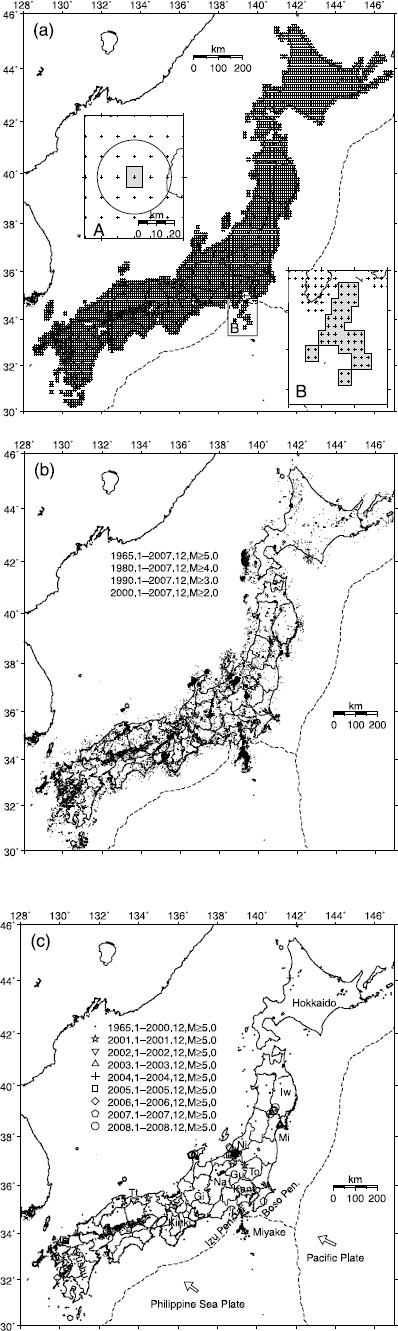

  

  (a) Calculation grids that covers Japan with spacing of 0.1°. Circle and shaded rectangle in inset map A indicate examples of a region for calculating model parameters and a forecast area, respectively. Shaded area near Miyake Island (labeled in Fig. 2(c)) in inset map B indicates the region excluded from the estimate of the nationwide mean b-value for tectonic reasons. (b) Epicenters of earthquakes used to make models. (c) Epicenters of target earthquakes with M ≥ 5.0. Different symbols correspond to different periods. Prefecture abbreviations: Iw, Iwate; Mi, Miyagi; Ni, Niigata; To, Tochigi; Gu, Gunma; Na, Nagano; Gi, Gifu; Tt, Tottori. White arrows indicate relative movements of the oceanic plates against the land plate.

• Step 2. We treated the “threshold magnitude” M_th in each region to be the magnitude bin that includes the largest number of events (Fig. 3). Note that because the JMA catalog rounds off magnitudes to the nearest tenth, M 2.1, for example, means the bin 2.05 ≤ M < 2.15, and M_th is not 2.1 but 2.05.

  Fig. 3.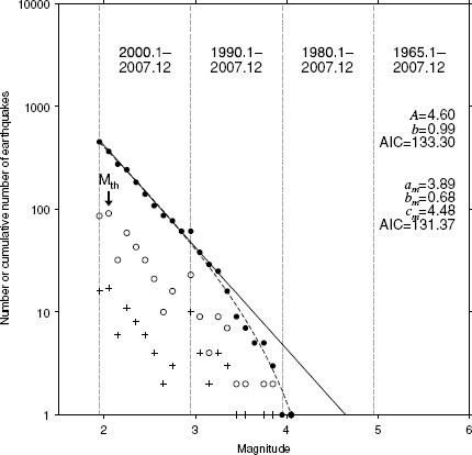

  

  Frequency-magnitude distribution within a radius of 20 km from the grid cell at lat 34.4°N, long 136.1°E. Data and symbols are the same as in Fig. 1. Distributions are approximated by two theoretical curves, the original G-R law (solid line) and the modified G-R law (dashed line). Estimated a- and b-values and AIC for the original G-R law and a _m -, b _m -, and c _m -values and AIC for the modified G-R law are shown on the right side.

• Step 3. We derived parameters for both the G-R and modified G-R law from the frequency-magnitude distribution in regions where the number of earthquakes in the virtual catalog with M ≥ M_th was at least 200. In regions with fewer than 200 such events, the b-value was assumed to be the mean b-value estimated by the G-R law for all earthquakes in the study region, excluding the area around Miyake Island (enclosed area in Fig. 2(a)) because events in that region were tecton-ically different, as discussed in Section 7.6.

• Step 4. We compared AIC values for the G-R and modified G-R laws for the frequency-magnitude distribution in each region and selected the law that yielded the smaller value. If the difference between the AIC values was less than 1, we selected the G-R law to reduce the risk of underestimating the probability (discussed further in Section 7.3). When calculating AIC values, we imposed conditions of one free parameter for the G-R law and two free parameters for the modified G-R law, because a- and a _m -values are treated as fixed values determined by the total number of earthquakes with M ≥ M_th.

• Step 5. To estimate the expected rate of earthquakes with M ≥ M_th in the testing period, we used the data from the final year in the modeling periods and estimated the a-value for the G-R law and a _m -value for the modified G-R law by taking the testing period length into account (Fig. 4(a)). When a large earthquake closely preceded the testing period (earthquakes with M ≥ 5.0 within one year or M ≥ 7.0 within five years), we forecasted the expected seismicity by applying the modified Omori formula (Utsu, 1957) to the modeling data (Fig. 4(b)). When more than one such large earthquake occurred in a region, the largest (and the last if there are multiple largest events) one was assumed to be the mainshock. There were also cases in which a region included aftershocks but not a mainshock. However, if the maximum earthquake extracted in each region satisfied the above magnitude and period condition, aftershock activity was estimated the same way even if the maximum earthquake was not a true mainshock.

  Fig. 4.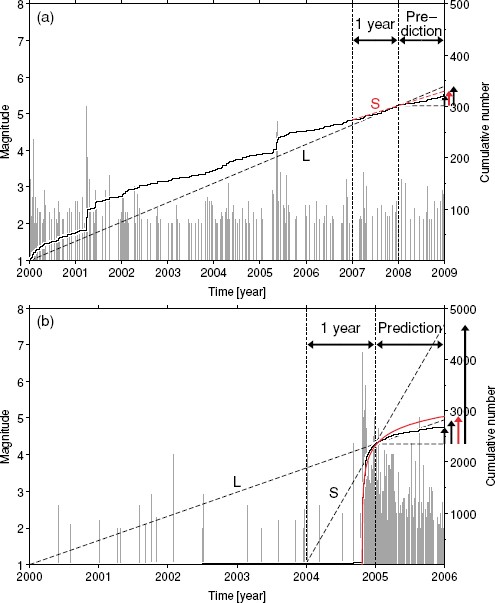

  

  Plot of magnitude and cumulative numbers of events versus time within a radius of 20 km from the grids at (a) lat 36.7°N, long 139.4°E and (b) lat 37.3°N, long 138.9°E. Lines L and S denote long-term and short-term seismicity rates, respectively. Red curve in (b) denotes aftershocks calculated by the modified Omori formula with parameters K_a = 458.37, c_a = 0.26, and p = 1.07. These parameters are obtained for the period from the mainshock to the end of 2004.

• Step 6. Finally, we used the obtained parameters to estimate the seismicity rate for a range of M(5.0 ≤ M ≤ 9.0) in the testing periods. The forecast area corresponding to each grid cell was defined as an outline of 0.1° × 0.1° in latitude and longitude centered at each grid (inset map A in Fig. 2(a)). As a region for calculating model parameters was circular while a forecast area was rectangular, the expected seismicity rate for a forecast area was corrected by taking into account the ratio of a rectangular area to circular one. The locations of target earthquakes were represented by epicenters without considering the size of their source area.

4.2 Minimum limit of seismicity rate

When no earthquake with M ≥ M _th occurred in the modeling data in a region, the expected seismicity rate of target earthquakes could not be obtained because the a-value in the G-R law and a _m -value in the modified G-R law could not be estimated. To estimate such low seismicity rates in some regions, we adopted the following assumption. The Earthquake Research Committee (2006) proposed that the average displacement rate for active faults of grade C, the lowest class of activity, is 0.024 mm/y. We assumed that the average displacement rate is 1/10 of this rate, 0.0024 mm/y, in grid cells where seismicity is too low to be estimated from seismicity data. Matsuda (1975) derived an empirical relation of displacement D (m) and M given by log D = 0.6M−4.0, and by extrapolation, displacement D for M 5.0 is 0.1 m. Thus, an earthquake of M 5.0 would occur once in about 42,000 years (2.4 × 10⁻⁵/y) for an average displacement rate of 0.0024 mm/y. Then we estimated minimum limits of seismicity rate for each M bin between 5.0 and 9.0 from the G-R law and the b-value for each grid cell.

Note that we assumed that the minimum limit of seismicity rate mentioned above is applicable to earthquakes with M ≥ c _m , and we estimated the minimum rate for each M bin from the G-R law with the mean b-value.

5. Statistical Evaluation of Earthquake Forecast Models

We evaluated the proposed earthquake forecast models statistically by using a log-likelihood test and an N-test (Kagan and Jackson, 1995; Schorlemmer et al., 2007).

5.1 Log-likelihood evaluation

We evaluated the models by comparing the log-likelihood of the models for the observed target earthquake distribution. We divided the target area and the earthquake magnitudes into a three-dimensional grid of K cells in which the third dimension is magnitude. When earthquakes occur independently in each cell, the probability P _ij that an earthquake, whose average occurrence rate (Poisson rate) is λ in the cell, occurs just k times is expressed by the Poisson process in the form

(4)

where the subscript i indicates grid number (1 to 5483) and j indicates the index of the target magnitude (1 to 41, corresponding to steps of 0.1 magnitude from M 5.0 to M 9.0), for a total number of cells K = 5483 × 41 = 224,803. The log-likelihood (lnL) for all cells is obtained by

(5)

As P _ij is not larger than 1, the closer to zero that ln L approaches, the more accurate the model becomes.

5.2 N-test

The N-test is a statistical method to check the consistency in occurrence numbers between observed earthquakes and predicted ones (Kagan and Jackson, 1995; Schorlemmer et al., 2007). Assuming the Poisson rate (average seismicity rate) for the J th cell in the forecast period to be λ _J (where J = 1,2,…, K), the expected number of earthquakes in the cell, E[n _J ], is given by

(6)

Thus the total expected number in all cells, E[n], is given by summation of the Poisson rate in each cell:

(7)

As the total expected number follows the Poisson distribution with the Poisson rate E[n], the confidence interval corresponding to an arbitrary significance level can be estimated easily. We used a significance level of 95% in this study. It should be noted that the N-test does not evaluate the spatial distribution of the number yielded by a model. For example, when a model forecasts five earthquakes in western Japan and none in eastern Japan, and five actual earthquakes occurred only in eastern Japan, the N-test does not reject the model. Therefore, we used the N-test results only for reference in this study.

6. Results

6.1 MGR model

Figure 5 shows the expected number of earthquakes with 5.0 ≤ M ≤ 9.0 for each year forecasted by the MGR model on the basis of the catalog from 1965 to the end of the previous year. The results for 2008 (based on the 1965–2007 catalog), for example, are separated into three regions in Fig. 6 according to the G-R law that was applied: the G-R law with variable b, the modified G-R law, and the G-R law with constant mean b. Table 1 lists the number of grid cells for each G-R law and the results of the log-likelihood and N-tests. For forecast year 2008, for example (Fig. 5(h) and Fig. 6), the G-R and modified G-R laws could be distinguished and applied in 2038 of the 5483 grid cells because the number of earthquakes in these cells was atleast 200 (step 3 in Section 4.1). The frequency-magnitude distribution followed the G-R law in 1653 of these cells and the modified G-R law in the other 385 cells through step 4 in Section 4.1. The number of target earthquakes expected by the MGR model was large in Niigata prefecture, Nagano-Gifu prefecture, eastern Izu peninsula, Kinki district, and central Kyushu district (Fig. 5(h) and Fig. 6(a) and 6(b); see Fig. 2(c) for place names) because the seismicity rate is high or the b-value is small in these regions. Similar features are seen for the other forecast years (Fig. 5).

Fig. 5.

Distributions of expected numbers of earthquakes with 5.0 ≤ M ≤ 9.0 predicted by the MGR model for (a) 2001, (b) 2002, (c) 2003, (d) 2004, (e) 2005, (f) 2006, (g) 2007, and (h) 2008 using data from 1965 to the year before each forecast period. Symbols for each figure are the same as in Fig. 2(c).

Table 1.

Retrospective forecasts by the MGR, Vbv, and Cbv models using a radius of 20 km. In the column “Number of grid cells,” 1, 2, and 3 indicate regions where the G-R law with variable b-values, the modified G-R law, and the G-R law with constant b-value are applied, respectively. Underlined numbers in the “log likelihood” column indicate the best log likelihood among the three models in each forecast period. In the “N-test” column, E[n] and N indicate the expected and actual numbers of target earthquakes in the forecast periods, respectively; entries marked with an “x” are rejected models with 95% significance level.

Four earthquakes with M ≥ 5.0 occurred in 2008: the mainshock (M 7.2) called the Iwate-Miyagi Nairiku earthquake and three of its aftershocks (M 5.7, M 5.3, M 5.2). Frequency-magnitude distributions in the grid cells where the M 7.2, M 5.3, and M 5.2 events occurred followed the G-R law and yielded b-values of 0.81, 0.63, and 0.87, respectively, which are smaller than or equal to the nationwide mean b-value of 0.87. For the grid cell of the M 5.7 event, the frequency-magnitude distribution followed the modified G-R law, and c _m was estimated at 6.3. The expected seismicity rates for that year were 0.4594 × 10⁻⁵, 0.3518 × 10⁻³, 0.5159 × 10⁻³, and 0.1707 × 10⁻³ for the cells of the M 7.2, M 5.7, M 5.3, and M 5.2 events, respectively. Figure 6(d) shows the distribution of c _m in 385 cells. The estimated upper limits of c _m were lower in southern Hokkaido, southern Kinki district, and southern Kyushu district than in other regions. Regions where c _m was relatively high correspond to places where large earthquakes occurred during the modeling periods.

Fig. 6.

Forecast for 2008 by the MGR model using data from 1965 through 2007. Distributions of expected numbers of earthquakes with 5.0 ≤ M ≤ 9.0 for regions estimated by (a) the G-R law with variable b-values in each region, (b) the modified G-R law, and (c) the G-R law with a constant mean b-value. (d) Distributions of c _m values. Circles in (a) and (b) denote target earthquakes that occurred in the corresponding regions.

6.2 MGR model vs. Vbv model

Table 1 shows that the MGR model was generally superior to the Vbv model because the log-likelihood for the MGR model, which combines the G-R and modified G-R laws, was greater than that for the Vbv model, which uses only the G-R law and assumes the b-value will vary regionally. The difference between these models is in the use of the modified G-R law. The numbers of earthquakes expected by the MGR model in cells where the modified G-R law is applied are lower than those expected by the Vbv model (Fig. 7). Note that no target earthquakes with 5.0 ≤ M ≤ 9.0 occurred in those cells. As the expected seismicity rate for earthquakes larger than c _m was constrained to a minimum limit by the modified G-R law, the MGR model was superior to the Vbv model when target earthquakes did not occur in the grid cell.

Fig. 7.

Comparison of forecasts for 2002 by the MGR and Vbv models using data from 1965 through 2001. Expected numbers of earthquakes with 5.0 ≤ M ≤ 9.0 estimated by (a) the modified G-R law in the MGR model and (b) the Vbv model in the same regions as (a). (c) The difference between (a) and (b). (d) Distribution of c _m values.

There was one exceptional case in 2007 in which the Vbv model was superior to the MGR model for target earthquakes. An earthquake with M 5.2 occurred beneath the Boso Peninsula on August 18, 2007, where the modified G-R law was used in accordance with step 4 in Section 4.1. The estimated value of the upper magnitude limit c _m was 4.6, thus the occurrence of the M 5.2 earthquake made the MGR model perform worse than the Vbv model.

6.3 Vbv model vs. Cbv model

Comparing the log-likelihoods of the Vbv model, which used variable b-values in each region, and the Cbv model, which used a constant mean b-value for the whole study area, we found that the Cbv model was better than the Vbv model in five cases out of eight (Table 1). Although we expected the use of regional b-values to favor the Vbv over the Cbv model, the results did not show a clear tendency. Figure 8 shows an example of the forecasts for 2002 by the Vbv and Cbv models using data from 1965 through 2001. As seen in Table 1, the Cbv model was better than the Vbv model for 2002, mainly because an earthquake occurred in western Tottori prefecture where the expected number of events was relatively small (Fig. 8(c)) a result of the high b-value in that region (Fig. 8(d)).

Fig. 8.

Comparison of forecasts for 2002 by the Vbv and Cbv models using data from 1965 through 2001. Expected numbers of earthquakes with 5.0 ≤ M ≤ 9.0 estimated by (a) the G-R law with variable b-values in each region and (b) the Cbv model in the same regions as (a). (c) The difference between (a) and (b). (d) The difference of b-values between the Vbv and Cbv models. The triangle in (c) denotes a target earthquake that occurred in the region where the variable b-value is estimated.

The Vbv model was superior to the Cbv model for 2008 (Fig. 9). The expected number distribution in Fig. 9 is similar to that in Fig. 8. The Iwate-Miyagi Nairiku earthquake occurred in the forecast period. The Vbv model was better than the Cbv model because the number of earthquakes expected by the Vbv model was larger in the region where the M 5.7 aftershock occurred, because the estimated regional b-value was 0.50, which is smaller than the mean b-value (0.87), although the difference of expected numbers in the grid cell in the two models was very small (0.01/year).

Fig. 9.

Comparison of forecasts for 2008 by the Vbv and Cbv models using data from 1965 through 2007. Explanation is the same as for Fig. 8.

6.4 MGR model vs. Cbv model

The log-likelihoods in Table 1 show that the MGR model was better than the Cbv model in four of the eight cases, which means there is little difference between the performance of the models. From the other model comparisons in Sections 6.2 and 6.3, it might have been expected that the MGR model would be the best of the three models, but the superiority of the MGR model was not clear. We discuss ways to clarify this situation below.

7. Discussion

7.1 The effect of the radius of each region

To simplify the procedure, we adopted a constant region radius in this study. As the median target magnitude was M 7.0, we selected a region radius of 20 km, with an area almost equivalent to the focal size of an M 7.0 earthquake (Utsu and Seki, 1955). Because the number of earthquakes extracted from a region is small if its radius is small, the number of regions where the G-R and modified G-R laws could be discriminated (step 3 in Section 4.1) decreases at small radii. In addition, when the number of earthquakes is small, the estimation error of the parameters for the frequency-magnitude distribution becomes large and we cannot obtain stable results. On the other hand, if a large radius is selected, the estimated parameters represent spatially smoothed features that provide less information about the regional variation of seismicity. Tables 2 to 4 show results for radii of 10 km, 30 km, and 40 km, corresponding to M 6.4, M 7.3, and M 7.6 earthquakes, respectively. For a radius of 10 km, less than 1/10 of the grid cells (524 of 5483) are suitable for discriminating between the G-R and modified G-R laws (step 3 in Section 4.1). This proportion is about 1/4, 1/2, and 2/3 for radii of 20 km, 30 km, and 40 km, respectively. The results of the forecast change to some extent by changing a radius. For example, with a 10-km radius (Table 2), the MGR model is better than the Cbv model for 2001 but worse for 2006 based on the log-likelihood value, whereas the results are the opposite with a 20-km radius (Table 1).

Table 2.

Comparison of retrospective forecasts by the MGR, Vbv, and Cbv models using a radius of 10 km. See Table 1 for explanation.

Table 3.

Comparison of retrospective forecasts by the MGR, Vbv, and Cbv models using a radius of 30 km. See Table 1 for explanation.

Table 4.

Comparison of retrospective forecasts by the MGR, Vbv, and Cbv models using a radius of 40 km. See Table 1 for explanation.

In addition, in the forecast for 2008, the MGR model is better than the Vbv model for a 20-km radius (Table 1), but the results are reversed for a 30-km and 40-km radius (Tables 3 and 4). The reason is as follows. The M 7.2 Iwate-Miyagi Nairiku earthquake occurred on June 14, 2008. However, during the modeling period, seismicity was relatively high at locations 30 km southwest and 30–40 km south-southeast of the mainshock. Thus the region centered at lat 39.0°N, long 140.9°E includes both this seismicity and the mainshock if the radius is 30 km or 40 km, but not if the radius is 20 km. When the region includes this seismicity, the log-likelihood for the MGR model becomes small because the modified G-R law is selected and c _m is estimated at 6.9, which is less than the mainshock magnitude of 7.2.

When a radius of 40 km is selected, the total log-likelihood for the MGR model is largest, which indicates that we might have a choice to select a radius of 40 km instead of 20 km. The selection of radius is a difficult problem. It may be advantageous in future work to treat radius as a variable parameter, depending on the magnitude of the target earthquake or the location of the regions.

7.2 The effect of the modified G-R law

The log-likelihood values for the MGR model, which applies the modified G-R law to some regions, tend to be larger than those for the Vbv model, which uses only the G-R law (e.g. Table 1). Therefore the effect of introducing the modified G-R law into the forecast model is evident. The MGR model was worse only in the forecast for 2007 because the magnitude of the M 5.2 earthquake beneath the Boso Peninsula on August 18, 2007, exceeded the value of c _m , which was estimated at 4.6. In this region an M 4.9 earthquake that occurred on October 8, 1966, was excluded from our virtual catalog used for modeling because events less than M 5 were rejected during that period. Thus, introducing the modified G-R law may be risky for estimating c _m if the data period is not long enough. This problem may be avoidable in future work by setting a lower limit for c _m based on the largest earthquake in a long-term catalog. In addition, a forecast model incorporating the estimation error of c _m (Mabuchi et al., 2002) may yield better results.

On the other hand, Burroughs and Tebbens (2002, BSSA) found that an upper-truncated power law, which is equivalent to the modified G-R law, applied to earthquake cumulative frequency-magnitude distributions yields a time-independent scaling parameter called the α-value. By analyzing several types of seismicity, they showed the α-value for the short time intervals is equal to the b-value obtained by applying the G-R law to the entire record. This suggests that the modified G-R law is not necessarily applicable for a long term data and the G-R law using α-value instead of b-value derived from short term data might be useful for forecasting. The method using the α-value can be an alternative in the future work for a longer term prediction. However, from our result mentioned above, the introduction of the modified G-R law into the forecast model is obviously effective to improve the prediction as far as our tested forecasting period is concerned (seven years at most in Section 7.5). We consider that there exist some regions in inland Japan where a frequency-magnitude distribution exhibits a convex-upward curve rather than a straight line and departs from the G-R law by nature, or our forecasting period is short enough for the modified G-R law to become superior to the G-R law in regions where the modified G-R law is selected in the modeling period.

7.3 Model selection by AIC

Generally, a model having a smaller AIC should be selected when models are chosen on the basis of AIC. However, we selected the G-R law when the difference of AIC between the G-R and modified G-R laws was less than 1, as mentioned in Section 4.1, to reduce the risk of underestimating the probability. We assumed that no earthquake with M ≥ c _m will occur when the modified G-R law is applied to the region, and this assumption is a severe constraint. For example, AIC for the modified G-R law is smaller than that for the G-R law by 0.54 in the region where the Iwate-Miyagi Nairiku earthquake occurred (Fig. 10). Note that the data period in Fig. 10 is from 1930 through 2007. The value of c _m was estimated to be 5.7 by the modified G-R law, but a mainshock with M 7.2 occurred on June 14, 2008. In this case, the modified G-R law had a negative effect. Therefore, we decided to set a bias of AIC by 1 when selecting the G-R law, but it was a decision made for trial purposes rather than one arising from a rigorous analysis.

Fig. 10.

Frequency-magnitude distribution within a radius of 20 km from the grid at lat 39.0°N, long 140.9°E. Symbols are the same as in Fig. 1 except that M ≥ 5.0 in this case is for the period 1930–2007. Explanation is the same as for Fig. 3.

7.4 The effect of aftershocks

As mentioned in Section 4.1, when a large earthquake occurred closely preceding the forecast period, we forecasted the expected number of earthquakes with M ≥ M _th in the forecast period by using the modified Omori formula

(8)

where t is time after the mainshock, n(t) is the number of aftershocks per unit time, and K _a , c _a , and p are constants (Utsu, 1957). In this study, to simplify the procedure we took into account only mainshocks with M ≥ 5.0 within the preceding year or M ≥ 7.0 within the preceding five years. When there were no such mainshocks, we estimated the expected number in the forecast period from the seismicity rate in the year just before the forecast period. As shown in Fig. 4(b), models that make adjustments on the basis of the aftershock decay rate can avoid overestimating the seismicity in forecast periods.

Generally it may be better to account for aftershock activity added to the background seismicity in the form

(9)

where S_b is the background seismicity rate. Theoretically, if we apply Eq. (9) to the modeling data, we can estimate the background seismicity as well as the aftershock activity and expect to forecast future seismicity more appropriately. However, if the data are insufficient, Eq. (9) is not necessarily a good selection. For example, when we apply Eqs. (8) and (9) to aftershocks of the Iwate-Miyagi Nairiku earthquake (M 7.2) of June 14, 2008, and estimate parameters using data between the mainshock and the end of 2008, the result of Eq. (8) is a better match to the actual activity for 2009 than the result of Eq. (9). Therefore, in this study we adopted Eq. (8) to evaluate the effect of aftershock activity.

7.5 The effect of forecast periods

Although forecast periods were fixed at one year or three years in accordance with the rule of CSEP for Japan, we tested the models for a wider range of periods. Comparing total log-likelihood values of three models in Tables 1, 5, 6, and 7, we found that the MGR model shows a tendency to improve for longer forecast periods such as three, five, or seven years. The effect of setting regionally variable b-values in the MGR and Vbv models tends to become evident in longer term forecasts because the number of target earthquakes increase and we can get statistically more stable results. Note that there are some cases that result in worse N-test results for the three models if the forecast period includes a large number of earthquakes, as in the case of the Mid Niigata prefecture earthquake (M 6.8) of October 23, 2004, and its many aftershocks. We discuss this further in Section 7.9.

Table 5.

Comparison of retrospective forecasts by the MGR, Vbv, and Cbv models using a radius of 20 km and forecast period of 3 years. See Table 1 for explanation.

Table 6.

Comparison of retrospective forecasts by the MGR, Vbv, and Cbv models using a radius of 20 km and forecast period of 5 years. See Table 1 for explanation.

Table 7.

Comparison of retrospective forecasts by the MGR, Vbv, and Cbv models using a radius of 20 km and forecast period of 7 years. See Table 1 for explanation.

7.6 Seismicity near Miyake Island

Most of the target earthquakes in this study occurred in the continental crust. However, regions from the Izu Peninsula to Miyake Island belong to a volcanic arc on the Philippine Sea plate, and earthquakes in these regions occur in oceanic crust or mantle. Near Miyake Island, volcanic earthquakes began June 26, 2000, and in the next two months, a notable swarm of activity occurred, including more than 7200 events with M ≥ 2.8 (= M _th ), more than 870 with M ≥ 4.0, 78 with M ≥ 5.0, and 6 with M ≥ 6.0 (of which the two largest were M 6.5). This activity is equivalent to the aftershock sequence of an M 8 class mainshock. However, it damped rapidly, and the average number of earthquakes with M ≥ 2.8 was around 20 per year from 2003 through 2008.

As this swarm was related to magmatic activity in oceanic crust and mantle, its characteristics might be very different from the on-land events that were our main target. Therefore, we excluded the Miyake Island region when we estimated a nationwide mean b-value from seismicity in the study area (Fig. 2(b)). This b-value was also used as the default in regions where the G-R and modified G-R laws could not be distinguished (step 3 in Section 4.1), including near Miyake Island.

7.7 Effect of minimum seismicity rate

As mentioned in Section 4.2, we assumed that target grid cells have a minimum rate of seismicity for earthquakes with M > c _m . We presumed that an earthquake of M 5.0 will occur once in about 42,000 years (2.4 × 10⁻⁵/y) as the minimum rate. But we also examined cases in which an earthquake of M 5.0 will occur once in 4,200 years (2.4 × 10⁻⁴/y) or 420,000 years (2.4 × 10⁻⁶/y). The results are shown in Tables 8 and 9 for a radius of 20 km and forecast period of one year. The log-likelihood changes to a small extent, but only for the 2006 forecast did it change the rank order of the different models.

Table 8.

Comparison of retrospective forecasts by the MGR, Vbv, and Cbv models using a radius of 20 km and a minimum seismicity rate for M 5.0 of 2.4 × 10^×/y. See Table 1 for explanation.

Table 9.

Comparison of retrospective forecasts by the MGR, Vbv, and Cbv models using a radius of 20 km and a minimum seismicity rate for M 5.0 of 2.4 × 10⁻⁶/y. See Table 1 for explanation.

7.8 Long-term or short-term data for seismicity estimations

As mentioned in Section 4.1, we estimated the seismicity rates from the data for the year just before the testing period. There is an advantage in using a long data record for estimating parameters b, b _m , and c _m , because the estimation error is expected to decrease as the number of earthquakes increases. On the other hand, long-term data may be a disadvantage for estimating parameters a and a _m because seismicity rates fluctuate over relatively short periods. For example, in Fig. 4(a), the expected seismicity is expressed by line L for long-term data and line S for short-term data, and the latter is a better fit in prediction. Therefore, for short-term forecasts such as one or three years, as proposed in CSEP for Japan, we estimated the expected seismicity rate from the last year of data in the modeling period.

7.9 Effect of definition of target earthquakes

Aftershocks cannot be forecasted by our models because they assume that earthquakes occur independently and do not consider triggering effects. However, as aftershocks are also targeted in the forecast experiment by CSEP for Japan, the results listed in Tables 1 to 9 are for target earthquakes including aftershocks, which makes results worse when many aftershocks occur. For example, the Mid Niigata prefecture earthquake (M 6.8) occurred on October 23, 2004, and 26 aftershocks with M ≥ 5.0 occurred by the end of 2004. In the N-test, the MGR model expected 5.62 target earthquakes in 2004 whereas 28 earthquakes were observed: the Mid Niigata prefecture earthquake, its aftershocks, and one earthquake in western Hokkaido on December 14, 2004. In addition, the log-likelihood was worse for 2004 than that for other forecast years. Table 10 shows that when target earthquakes were restricted to main-shocks, the total expected number E[n] and total observed number in the N-test were similar to each other, and the log-likelihood was near the same level as the other forecast years. The definition of target earthquakes is essential for evaluation of models. It is significant that the models in this study were intended to forecast mainly mainshocks, which differs from the framework of CSEP for Japan.

Table 10.

Comparison of retrospective forecasts by the MGR, Vbv, and Cbv models using a radius of 20 km and target earthquakes that are exclusively mainshocks. See Table 1 for explanation. The five periods shown in boldface in the first column have had aftershocks removed from target earthquakes in each forecast period.

7.10 Future problems

The models in this study were designed to forecast target earthquakes with 5.0 ≤ M ≤ 9.0 and depth ≤ 30 km by using only seismicity data after January 1965, according to the framework of CSEP for Japan. We ignored all information about tectonic settings (except in the case of Miyake Island), geodetic crustal movements, velocity structure in the crust, spatial distribution of active faults, physical mechanism of earthquakes, and so on, all of which are related to seismicity. To improve the models, it is important to bring this information into them. For example, considering tectonic information, in the Kanto district both continental and oceanic crust interact beneath the Boso Peninsula, thus it is reasonable to treat the crustal types separately by considering the distribution of hypocenters rather than epicenters.

For another example, recently it has been suggested that earthquakes in the continental crust are related to melts in the lower crust (Okada et al., 2008). Our model might be improved by clarifying the relationship between seismicity and velocity structure in the lower crust. We consider the models proposed here to be basic models that can be improved by adding more information.

8. Summary

We proposed earthquake forecast models based on the G-R law or the modified G-R law and compared their performance by retrospective forecast. The results are as follows:

• 1. The MGR model, using both the modified G-R and G-R laws, was better than the Vbv model, using only the G-R law.

• 2. The Cbv model, based on a spatially constant b-value, was better than the Vbv model, based on regionally variable b-values for short-term (one year) forecasts.

• 3. The difference between the MGR and Cbv models was not clear for short-term forecasts.

• 4. The MGR and the Vbv models, using regionally variable b-values, tended to become better than the Cbv model for long-term (three years or longer) forecasts.

On the basis of our results, we propose the use of the MGR model for CSEP for Japan.

References

Akaike, H., A new look at the statistical model identification, IEEE Trans. Auto. Cont., 19(6), 716–723;, 1974.
Aki, K., Maximum likelihood estimate of b in the formula logN = a−bM and its confidence limits, Bull. Earthq. Res. Inst., 43, 237–723;239, 1965.
Anderson, R. N., A. Hasegawa, N. Umino, and A. Takagi, Phase changes and the frequency-magnitude distribution in the upper plane of the deep seismic zone beneath Tohoku, Japan, J. Geophys. Res., 85, 1389–723;1398, 1980.
Burroughs, S. M. and S. T. Tebbens, The upper-truncated power law applied to earthquake cumulative frequency-magnitude distributions: Evidence for a time-independent scaling parameter, Bull. Seismol. Soc. Am., 92, 2983–723;2993, 2002.
Earthquake Research Committee, Report: ‘National Seismic Hazard Maps for Japan’, 2006 (in Japanese).
Gerstenberger, M., S. Wiemer, and D. Giardini, A systematic test of the hypothesis that the b value varies with depth in California, Geophys. Res. Lett., 28, 57–60, 2001.
Gutenberg, B. and C. F. Richter, Frequency of earthquakes in California, Bull. Seismol. Soc. Am., 34, 185–188, 1944.
Hirose, F, A. Nakamura, and A. Hasegawa, b-value variation associated with the rupture of asperities: Spatial and temporal distributions of b-value east off NE Japan, J. Seismol. Soc. Jpn., 2, 55, 249–260, 2002a (in Japanese with English abstract).
Hirose, F, A. Nakamura, J. Nakajima, and A. Hasegawa, Along-arc variation of magma source in the subducted slab beneath the NE Japan arc: Estimation from b-value and S-wave velocity distributions, J. Volcanol. Soc. Jpn., 47, 475–480, 2002b (in Japanese with English abstract).
Kagan, Y. Y. and D. D. Jackson, New seismic gap hypothesis: Five years after,J. Geophys. Res., 100, 3943–3959, 1995.
Mabuchi, H., M. Ohtake, and H. Sato, Global distribution of maximum earthquake magnitude M c based on a modified G-R model of magnitude-frequency distribution,J. Seismol. Soc. Jpn., 2, 55, 261–273, 2002 (in Japanese with English abstract).
Matsuda, T., Magnitude and recurrence interval of earthquakes from a fault, J. Seismol. Soc. Jpn., 2, 28, 269–283, 1975 (in Japanese with English abstract).
Murru, M., C. Montuori, M. Wyss, and E. Privitera, The locations of magma chambers at Mt. Etna, Italy, mapped by b-values, Geophys. Res. Lett., 26, 2553–2556, 1999.
Nanjo, K., H. Tsuruoka, N. Hirata, and Research group “Earthquake Forecast System based on Seismicity of Japan” Earthquake forecast testing experiment for Japan: Advancing the preparatory process towards the formal start of the experiment, Prog. Abst. Seismol. Soc. Jpn. 2009, Fall Meet., D22-01, 2009 (in Japanese).
Okada, T., S. Hori, T. Kono, T. Nakayama, S. Hirahara, K. Nii, A. Omu-ralieva, J. Nakajima, N. Umino, and A. Hasegawa, Inhomogeneous seismic velocity structure and its relation with seismic activity in the central part of Tohoku, NE Japan, Abst. Jpn. Geosci. Union Meet. 2008, S147-008, 2008.
öncel, A. O. and M. Wyss, The major asperities of the 1999 Mw = 7.4 Izmit earthquake defined by the microseismicity of the two decades before it, Geophys. J. Int., 143, 501–506, 2000.
Rydelek, P. A. and I. S. Sacks, Testing the completeness of earthquake catalogs and the hypothesis of self-similarity, Nature, 337, 251–254, 1989.
Scholz, C. H., The frequency-magnitude relation of microfracturing in rock and its relation to earthquakes, Bull. Seismol. Soc. Am., 58, 399–415, 1968.
Schorlemmer, D., S. Wiemer, and M. Wyss, Variations in earthquake-size distribution across different stress regimes, Nature, 437, 539–542, doi:10.1038/nature04094, 2005.
Schorlemmer, D., M. C. Gerstenberger, S. Wiemer, D. D. Jackson, and D. A. Rhoades, Earthquake likelihood model testing, Seismol. Res. Lett., 78, 17–29, 2007.
Suyehiro, S., Difference between aftershocks and foreshocks in the relationship of magnitude to frequency of occurrence for the great Chilean earthquake of 1960, Bull. Seismol. Soc. Am., 56, 185–200, 1966.
Umino, N. and I.S. Sacks, Magnitude-frequency relations for northeastern Japan, Bull. Seismol. Soc. Am., 83, 1492–1506, 1993.
Utsu, T., Magnitude of earthquakes and occurrence of their aftershocks, J. Seismol. Soc. Jpn., 2, 10, 35–45, 1957 (in Japanese with English abstract).
Utsu, T., A three-parameter formula for magnitude distribution of earthquakes, J. Phys. Earth, 22,71–85, 1974.
Utsu, T. and Y Ogata, Computer program package: Statistical Analysis of point processes for Seismicity, SASeis, IASPEI Software Library for personal computers, the International Association of Seismology and Physics of Earth’s Interior in collaboration with the American Seismological Society,6, 13–94, 1997.
Utsu, T. and A. Seki, A relation between the area of after-shock region and the energy of main-shock, J. Seismol. Soc. Jpn., 2, 7, 233–240, 1955 (in Japanese with English abstract).
Wessel, P. and W. H. F Smith, Free software helps map and display data, Eos Trans. AGU, 72, 441, 1991.
Wiemer, S. and J. P. Benoit, Mapping the b-value anomaly at 100 km depth in the Alaska and New Zealand subduction zones, Geophys. Res. Lett., 23, 1557–1560, 1996.
Wiemer, S. and S. R. McNutt, Variations in the frequency-magnitude distribution with depth in two volcanic areas: Mount St. Helens, Washington, and Mt. Spurr, Alaska, Geophys. Res. Lett., 24, 189–192, 1997.
Wiemer, S. and D. Schorlemmer, ALM: an asperity-based likelihood model for California, Seismol. Res. Lett., 78, 134–140, 2007.
Wiemer, S. and M. Wyss, Mapping the frequency-magnitude distribution in asperities: An improved technique to calculate recurrence times?, J. Geophys. Res., 102, 15115–15128, 1997.
Wyss, M., Changes of mean magnitude of Parkfield seismicity: A part of the precursory process?, Geophys. Res. Lett., 17, 2429–2432, 1990.
Wyss, M., D. Schorlemmer, and S. Wiemer, Mapping asperities by minima of local recurrence time: San Jacinto-Elsinore fault zones, J. Geophys. Res., 105,7829–7844, 2000.
Acknowledgments
We thank all the institutions, universities, and JMA for providing the unified hypocenter catalog. We also thank T. Utsu and Y. Ogata for the use of the SASeis program (Utsu and Ogata, 1997) to estimate parameters of aftershocks. This manuscript was greatly improved by careful reviews of two anonymous reviewers. Figures were prepared using GMT (Wessel and Smith, 1991).
Author information
Authors and Affiliations
Corresponding author
Rights and permissions
Open Access This article is licensed under a Creative Commons Attribution 4.0 International License, which permits use, sharing, adaptation, distribution and reproduction in any medium or format, as long as you give appropriate credit to the original author(s) and the source, provide a link to the Creative Commons licence, and indicate if changes were made.
The images or other third party material in this article are included in the article’s Creative Commons licence, unless indicated otherwise in a credit line to the material. If material is not included in the article’s Creative Commons licence and your intended use is not permitted by statutory regulation or exceeds the permitted use, you will need to obtain permission directly from the copyright holder.
To view a copy of this licence, visit https://creativecommons.org/licenses/by/4.0/.
About this article
Cite this article
Hirose, F., Maeda, K. Earthquake forecast models for inland Japan based on the G-R law and the modified G-R law. Earth Planet Sp 63, 239–260 (2011). https://doi.org/10.5047/eps.2010.10.002
Received:
Revised:
Accepted:
Published:
Issue Date:
DOI: https://doi.org/10.5047/eps.2010.10.002