Gravity changes associated with variations in local land-water distributions: Observations and hydrological modeling at Isawa Fan, northern Japan

Abstract

Gravity changes associated with variations in local land-water distributions have been observed at Isawa Fan in northern Japan, and modeled by hydrological equations. We solve the Richards equation numerically for the time variation in the vertical soil moisture distribution, which is then spatially integrated to estimate gravity changes due to the soil moisture distribution. In modeling Isawa Fan, we assume a simple hydrological model: a horizontally homogeneous soil in an infinite half-space. The estimated gravity is consistent with the observed gravity during a 50-day period within about 0.4 µgal root mean square, owing to both observed soil parameter values and the observation building geometry being incorporated into the hydrological model. However, the estimated gravity cannot fully reproduce annual gravity changes observed during a 2-year time frame, because the boundary conditions in the modeling determine only local water distributions and the resultant short-period gravity changes. Instead, the observed gravity over these 2 years can be reproduced within about 1.0 µgal root mean square, if the additional parameters of the annual gravity change (A_ac and A_as) and the snowfall effect (A_s) are calculated by the function regression to the observed gravity with the least-squares method. The hydrological modeling techniques presented here can be utilized at all gravity sites in flat areas similar to Isawa Fan, such that hydrological effects in gravity data can be corrected and mass transfers associated with earthquakes and volcanoes can be monitored.

1. Introduction

Observing changes in gravity is one of the most powerful methods for detecting mass redistributions associated with solid-earth tectonics, such as those resulting from earthquakes and volcanism (Furuya et al., 2003; Imanishi et al., 2004). However, gravity measurements are also sensitive to changes in land-water distributions in the vicinity of gravimeters. These changes originate from precipitation, snow cover, soil water infiltration, groundwater flow, river runoff and variations in the water level of oceans and lakes (e.g., Sato et al., 2001; Van Camp et al., 2006; Kazama and Okubo, 2009; Christiansen et al., 2011). To detect the minute gravity changes associated with solid-earth tectonics, water distribution effects in the original gravity data must be corrected to a high accuracy.

Many scientists have modeled the effects of land-water distribution on the observed gravity (e.g., Francis et al., 2004; Abe et al., 2006; Boy and Hinderer, 2006; Meurers et al., 2007; Jahr et al., 2009; Leirião et al., 2009; Longuevergne et al., 2009; Nawa et al., 2009; Pfeffer et al., 2011). For example, Hanada et al. (1990) found a simple proportional relationship between water level and absolute gravity (coefficient: +16 µgal/m) observed at Isawa Fan, northern Japan. Imanishi et al. (2006) reproduced land-water distribution effects observed at Matsushiro, central Japan, with an empirical tank model, assuming an instant gravity response to precipitation of −0.040 µgal/mm and a linear gravity recovery after precipitation of +3 × 10⁻⁶µgal/s. Wziontek et al. (2009) explained a seasonal gravity change of ∼10 µgal peak-to-peak at superconducting gravity stations in Europe by attraction and loading effects attributable to global land-water distributions. Creutzfeldt et al. (2010a, b) reproduced a non-tidal gravity change of ∼10 µgal in amplitude at Wettzell, Germany, by using spatial integrations of local water distributions observed with a lysimeter and borehole moisture meters.

However, the following three shortcomings exist in previous studies when estimating the effect on gravity due to land-water distributions. Firstly, the majority of models, including the tank model, assume a linear gravity response to precipitation (e.g., Hanada et al., 1990; Imanishi et al., 2006; Nawa et al., 2009; Lampitelli and Francis, 2010). Since water flow is governed by non-linear equations (as demonstrated in this study), there are limitations in applying linear theory to gravity responses (Kazama et al., 2005). Secondly, empirical methods can over- or under-estimate gravity amplitudes resulting from land-water distribution, because empirical methods only fit simple regression curves to observed gravity data (e.g., Bower and Courtier, 1998;

Harnisch and Harnisch, 2006). To reproduce the gravity response to water distribution, the distribution should be estimated by applying hydrological modeling, independently of observed gravity data. Thirdly, regional and global water storages have often been reproduced rather than local water storage (e.g., Sato et al., 2001; Boy and Hinderer, 2006; Neumeyer et al., 2006). Meanwhile, a number of studies report that the dominant area for land gravity observation is within a several hundred meter radius surrounding a gravimeter (e.g., Hasan et al., 2006; Kazama and Okubo, 2009), since gravity (i.e., the integral of the gravitational force) has a high sensitivity to mass in the vicinity of gravimeters (see Eq. (17)). Therefore, it is important to observe and model water distributions near these gravimeters, assuming a local hydrological model.

Taking these aspects into account, hydrological nonlinear equations should be solved directly for local water distributions and the consequent gravity change. Previous studies have utilized the hydrological equations (e.g., Abe et al., 2006; Hasan et al., 2008; Kazama and Okubo, 2009; Krause et al., 2009; Leirião et al., 2009; Naujoks et al., 2010), although all still show problems relating to the re-producibility of changes in gravity. For example, Abe et al. (2006) found that soil-water effects, estimated by a soil moisture retention function, corresponded to 80% of the observed instant gravity change during rainfall events in Bandung, Indonesia. However, the length of time for estimating the gravity was within only a single day during the rainfall events, because Abe et al. focused on short-period soil water infiltration within several meters from the gravimeter. To reproduce gravity responses over a longer period (i.e., more than one day), both a large-scale computation area and a long-period water distribution change must be taken into account. Kazama and Okubo (2009) found that gradual decreases in gravity after rainfall events, estimated through hydrological non-linear equations were, within the observation error, consistent with the gravity observed at the Asama volcano (in central Japan). However, the estimated amplitude for the instant gravity increase during rainfall corresponded to only 75% of the observed gravity, possibly owing to poor reproducibility of water distributions in the undulating volcanic region. Therefore, the method proposed by Kazama and Okubo (2009) should first be applied to an area having a simple topography (i.e., a plain), in order to test the correctness of their model.

In addition, for an accurate estimation of local water distributions and consequent gravity changes, hydrological and meteorological data must be collected near gravimeters. Researchers have carried out electrical resistivity surveys (Van Camp et al., 2006), lysimeter measurements (Creutzfeldt et al., 2010a), and borehole-core sampling (Creutzfeldt et al., 2010b), to understand, in detail, depth-dependent water distributions below the ground surface; however, such depth profile data is not available for all gravity observation sites, mainly because of financial limitations. A different approach is to realize that the bulk of the water mass distribution occurs in the uppermost ground layers, because soil pores and free spaces at the ground surface can preserve significant amounts of water in the form of soil water and snow (e.g., Sato et al., 2006). Therefore, it is vital to collect hydrological and meteorological data, such as precipitation, soil moisture and unconfined groundwater height, at the shallowest part of the ground in order to understand the gravity changes due to land-water distributions.

Thus, we are motivated to observe and model local land-water distributions near gravimeters in flat areas, with the aim of reproducing hydrological gravity changes accurately by applying hydrological modeling. Hydrological and meteorological data, in addition to gravity, are observed continuously within a radius of 50 m at Isawa Fan (Iwate Prefecture, northern Japan). In this research, a non-linear soil water diffusion equation (the so-called Richards equation; Richards, 1931; Kazama and Okubo, 2009) is solved to find the spatiotemporal soil water distribution, and this is spatially integrated to estimate the gravity change. The estimated change in gravity is shown to be consistent with a 50-day gravity change observed by a superconducting gravimeter (Crossley et al., 1999; Goodkind, 1999), within about 0.4 µgal root mean square (RMS).

2. Observations at Isawa Fan

Isawa Fan is located in the southern part of Iwate Prefecture, northern Japan (Fig. 1). This alluvial fan is one of the largest in Japan, and its radius and area are about 20 km and 200 km², respectively. In the central part of the fan is Mizusawa VLBI (Very Long Baseline Interferometry) Observatory (denoted by the small star in Fig. 1); one of the observatories belonging to the National Astronomical Observatory of Japan (NAOJ). This observatory measures and records geodetic, hydrological and meteorological data, in order to monitor minute ground deformations and their relation to water distribution changes (Okuda et al., 1974; Ooe and Hanada, 1982; Hanada et al., 1990). In December 2008, a superconducting gravimeter (type: TT70; serial number: #007) was moved from NAOJ Esashi Earth Tides Station (square in Fig. 1) to Mizusawa VLBI Observatory, for the detection of gravity changes due to local events at Mizusawa, including variations in land-water distributions (Tamura et al., 2009). On 23 January, 2009, the gravimeter started to observe continuous changes in gravity on the basement rock of the gravity observation building (Fig. 2), which had previously been used for absolute gravity observations (e.g., Okuda et al., 1974).

Fig. 1

Spatial distribution of observatories at Isawa Fan. The dashed line shows the approximate shape of Isawa Fan (radius: ∼20 km). The star, circle, triangle, diamond and square show the positions of the NAOJ Mizusawa VLBI Observatory, Suginodo Spring, Otemachi snow observatory, AMeDAS Esashi Observatory and NAOJ Esashi Earth Tides Station, respectively. Two squares—MF1 and MF2—, beach-ball-like circle and square DF show coseismic faults, focal mechanism and afterslip fault for the 2008 Iwate-Miyagi Nairiku Earthquake (Ohta et al., 2008; Iinuma et al., 2009; Suzuki et al., 2010). Digital elevation model SRTM30_PLUS (Becker et al., 2009) is used for surface elevation, and contours are drawn every 200 m. The large star in the bottom-right map shows the position of Isawa Fan in the northern part of Japan.

Fig. 2

Geometry of superconducting gravimeter (SG) in NAOJ Mizusawa Observatory. (Top) Overhead view of SG (circle) and the observation building (thick line). (Bottom-left) Cross-sectional view of SG (pentagon) and the observation building (thick line) along the east-west line. (Bottom-right) Approximate profile of the soil moisture below the ground surface.

Figure 3 shows data observed at Mizusawa Observatory during the period 2008 to 2010. The black bar in Fig. 3(a) and the thin solid line in Fig. 3(b) are the daily and annual precipitations, respectively. This precipitation data (original precipitation resolution: 0.5 mm; time resolution: 60 s) was observed with a tipping bucket rain gauge, belonging to a weather station located 50 m north of the gravity station. Note that fallen snow in winter was counted as equivalent liquid water, since the rain gauge has snow-melting equipment. The daily precipitation, R(t), from 2008 to 2010 was less than 55 mm/day, and the total precipitation, R_tot(t), in each year was 907.0 (in 2008), 1073.5 (in 2009) and 1151.5 mm (in 2010). These annual precipitation values are consistent with the average annual precipitation measured at AMeDAS (Automated Meteorological Data Acquisition System) Esashi Observatory (diamond in Fig. 1) of 1142.7 mm/year (Japan Meteorological Agency, 2011).

Fig. 3

Observed data at Isawa Fan from 2008 to 2010. Letters on the top horizontal axis denote initials of months, and the bottom horizontal axis shows days from 1 January 2008, Japan Standard Time (JST). (a) The solid bar is the observed daily precipitation, R(t), at Mizusawa, and the gray bar is Penman’s daily evapotranspiration, E(t), estimated from observed meteorological data at Mizusawa. (b) The thin solid line, dashed line and thick solid line are cumulative precipitation, R_tot(t), cumulative evapotranspiration, E_tot(t), and cumulative effective precipitation, P_tot(t), respectively. Gray bar is the observed depth of accumulated snow, S(t), at Otemachi (triangle in Fig. 1). (c) Solid line shows the average soil moisture variation, θ_obs(t), at 0–1 m below the ground surface observed at Mizusawa, and the gray area is the 1-σ error range of observed moisture, Δθ_obs(t). (d) Average water level change at Mizusawa with reference to ground surface level, h(t) − z_s(t). Gray and solid lines denote water level data observed with floating-type and pressure-type water level gauges, respectively. (e) Superconducting gravity data processed with BAYTAP-G (Tamura et al., 1991). Solid and gray lines are trend component, g_obs(t), and the irregular component (i.e., gravity observation noise).

The gray bar in Fig. 3(a) and the dotted line in Fig. 3(b) are the daily and annual evapotranspiration (as defined by Penman, 1948), respectively. The daily evapotranspiration, E(t), can be calculated (Miura and Okuno, 1993) from four daily meteorological data values (average air temperature, average relative humidity, sunlight hours and average wind speed) and four coefficients (psychrometer coefficient, latitude, anemometer height and ground surface albedo). Here, we used values for the above meteorological parameters observed at the weather station in Mizusawa observatory, and set the four coefficients as follows:

(1)

Note that an average albedo for soil and grass of 0.2 (Oke, 1978) was assumed in this study, even though in reality the ground surface albedo differs according to vegetation, soil color and moisture content (Idso et al., 1975; Betts and Ball, 1997; Post et al., 2000). The calculated E(t) varies from 0.5 mm/day (in winter) to 6 mm/day (in summer), and the total evapotranspiration, E_tot(t), in each year was 701.5 (in 2008), 698.7 (in 2009) and 715.0 mm (in 2010).

The thick solid line in Fig. 3(b) represents the total value of effective precipitation given by

(2)

Thus, P_tot(t) increases rapidly at precipitation events and decreases gradually between precipitation events. During the summer season in 2008, P_tot(t) fell below 0 mm because of the extremely low precipitation. The annual total values of effective precipitation were 205.5 (in 2008), 374.8 (in 2009) and 436.5 mm (in 2010).

Finally, the gray bars in Fig. 3(b) denote the snow depth at Otemachi (∼2.4 km northeast from the gravity observatory; triangle in Fig. 1), observed by the Iwate prefectural government (Iwate Prefecture, 2011). We utilized this data because the snow gauge at the weather station in Mizusawa Observatory was out of action during the measurement period. Snow accumulates in the region around Mizusawa Observatory from November to March every year, and its maximum depth during the three observation years was 27 cm on 21 February 2009.

Figure 3(c) shows the moisture content variation in m³/m³ near the weather station at Mizusawa Observatory, measured every 5 min with a soil moisture meter (Profile Probe PR2; Delta-T Devices Ltd.). This meter observes voltage changes at six sensors, and converts these voltages into an overall moisture change by using the conversion equation for organic soil (Miller and Gaskin, 1999). In this figure, θ_obs(t) (solid line) signifies the average moisture from the six observations at 0–1-m depth below the ground surface, and Δθ_obs(t) (gray envelope) is the 1-σ error range for the observed moisture. The absolute moisture value is 0.40 ∼ 0.55, and is consistent with the value found by a soil test (Grossman and Reinsch, 2002) of 0.51±0.04 on 8 November, 2008. θ_obs(t) increases sharply at rainfall events dependent on the amount of rain, and decreases exponentially after rainfall because of evapotranspiration and infiltration. However, the moisture level is approximately constant during the winter seasons (from December to April), suggesting that the covering snow blocks evapotranspiration from the soil surface and the covering snow provides moisture to the soil at a constant rate.

Figure 3(d) shows the average water table height, h(t), from the ground surface level, z_s; estimated from the water level variations of four shallow wells within 50 m of the gravity observatory. After 2 October, 2008, (solid line), the water height was measured with newly-installed water pressure gauges (Mini Diver DI-501; Schlumberger Ltd.), since the original data taken by floating water gauges (gray line) was often saturated when the change in water level exceeded the wire length between the float and pulley (as seen between June and July, 2008). The water table is located at a depth of 0.5–3 m below the ground surface, and rose steeply at precipitation events in synchronization with soil moisture increases. After precipitation events the water table reduced at an almost linear rate, because the unconfined ground-water was regularly pumped for domestic and agricultural use at Isawa Fan, and the groundwater flowed out eastward to the edge of Isawa Fan. (Water electrical conductivity at Suginodo Spring (circle in Fig. 1) is 220 µS/cm, about four times larger than that at Mizusawa wells (∼50 µS/cm), showing that the groundwater flows eastward at Isawa Fan under conditions of domestic and agricultural water pollution.)

Figure 3(e) plots the superconducting gravity data during the period 23 January, 2009, to 5 December, 2010. Gravity data was calculated from measured output voltages with a conversion coefficient of −56.082 [µgal/V] (Tamura et al., 2005), and divided into tidal, barometric, trend and irregular components by using the BAYTAP-G software package (Tamura et al., 1991). In addition, effects from the long-period tide, the polar motion and the arbitrary linear drift (−0.095 µgal/day) were corrected in the trend components. The solid and gray lines in Fig. 3(e) are the corrected trend component, g_obs(t), and the irregular component (i.e., the gravity observation noise), respectively. g_obs(t) is not shown between June and July, 2009, owing to a controller failure causing the noise amplitude and the g_obs(t) drift rate to be elevated. This failure was repaired by changing the controller on 27 July, 2009. g_obs(t) decreases by ∼10 µgal in two years, implying that instrumental drift was not fully removed from the observations. Furthermore, g_obs(t) increases quickly by a few microgals during precipitation events, in line with the soil moisture increase and water height rise (as seen for March 2009, October 2009, March 2010 and July 2010), suggesting that changes in the gravity signal are associated with corresponding changes in the land-water distribution.

Note that the 2008 Iwate-Miyagi Nairiku Earthquake (M_w 6.9) occurred in a southwestern area outside the Isawa Fan on 14 June, 2008. The coseismic slip at two main faults (labeled MF1 and MF2 in Fig. 1) reached a maximum of ∼3.5 m (Ohta et al., 2008), which triggered aseismic slip at the Detana Fault (DF in Fig. 1) of about 30 cm in the few months after the mainshock (Iinuma et al., 2009). The superconducting gravimeter at Mizusawa Observatory, however, did not detect any gravity change associated with these fault slips, because the gravimeter was installed about a half year after the earthquake event, and the aseismic slip effect cannot be separated from the instrumental drift in the superconducting gravity data.

3. Numerical Methods

Hydrologically, the near-surface crust consists of an un-saturated layer (or soil water layer), saturated layers (or groundwater layers, aquifers) and impermeable layers. In general, precipitated water: (1) falls onto the ground surface, (2) infiltrates vertically into the unsaturated layer as soil water, (3) reaches the water table of the unconfined aquifer, (4) flows horizontally into the unconfined aquifer as groundwater, and (5) discharges into rivers, lakes and the sea. If, for gravity changes, the water leakage at impermeable layers, and groundwater pumping from confined aquifers, are neglected, then the gravity change must be calculated from the spatiotemporal distributions of the soil water and the unconfined groundwater (Fig. 2).

The soil water distribution in the unsaturated layer can be estimated by using hydrological modeling (Jury and Horton, 2004; Kazama and Okubo, 2009). Conservation of water volume in the unsaturated layer can be written as

(3)

where θ = θ(z, t) and υ = υ(z, t) are the volumetric water content and vertical soil water velocity, respectively, at a vertical position z and a time t. Here, horizontal components, such as ∂υ/∂x and ∂υ/∂y, are neglected because the horizontal heterogeneity of soil water flow is assumed to be small for flat areas like Isawa Fan; in fact, the hydrological structure is thought to be horizontally homogeneous around Mizusawa VLBI Observatory, because the ground surface gradient around the observatory is only about 0.004 m/m, and groundwater is not pumped from both confined and unconfined aquifers in the area of the observatory (∼ 100 × 100 [m²]). Next, Darcy’s law is given by

(4)

where D(θ) and K(θ) are the vertical diffusivity and permeability, respectively, and depend exponentially on the water content, θ(z, t) (e.g., van Genuchten, 1980). A nonlinear diffusion equation (the Richards equation) is obtained by substitution of Eq. (4) into Eq. (3):

(5)

In this study, this equation was solved numerically for the spatiotemporal moisture distribution, θ(z, t), by using the finite difference method (FDM). For the FDM equations, the soil moisture for vertical cell i is θ _i , and a staggered grid (Aki and Richards, 1980) is used to express the moisture average, the spatial derivation of moisture and the flow velocity (Eq. (4)) as follows:

(6)

(7)

(8)

With these definitions, the non-linear diffusion equation (Eq. (5)) for the FDM expression is

(9)

where is the moisture value for position i at the next time step. This equation was solved for the spatiotemporal moisture distribution using Fortran code. For application to Isawa Fan, the vertical and time grid sizes were set as Δ z = 0. 05 [m] and Δt = 300 [s], respectively.

To find a realistic estimate for the soil water distribution in the FDM calculation, we defined two boundary conditions, an initial condition, and soil parameters, as follows.

• Vertical soil water velocity at the ground surface is set to be equal to the effective precipitation:

  

  (10)

  where z_s and p are the ground surface height above sea level (Fig. 2) and the infiltration capacity for the ground, respectively. The infiltration capacity p was set as 1.0 for the soil ground surface for this study, because all precipitation is considered to infiltrate into the soil unless the precipitation intensity exceeds 100 mm/h (Murai and Iwasaki, 1975).

• Water content at the saturated layer (z ≤ h(t))is fixed to be the maximum water content (i.e., effective ^porosity), θ_max:

  

  (11)

  Here, d is the depth of the computed region and was set equal to 10.0 m to satisfy the condition z_s − d ≤ h(t) for all times. In this study, the observed water height change, h(t) (Fig. 3(d)), was utilized to decide the position where the moisture is fixed to θ_max, and θ_max was observed with a test on soil sampled at the observatory (see Eq. (16)). Note that the horizontal groundwater flow in the unconfined aquifer is not modeled numerically in this study, because the effects of groundwater flow and its temporal change will be incorporated as this boundary condition into our hydrological modeling.

• A steady-state soil water distribution was assumed for the initial distribution of θ(z, t):

  

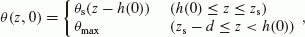  (12)

  where θ_s(Z) is the steady-state soil water distribution at a vertical height Z above the water table (Fig. 2). θ_s(Z) was estimated from the FDM calculations by continuing to apply an average effective precipitation P₀ onto the ground surface before the soil water distribution converges. Here, the average value of the effective precipitation was given by

  

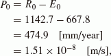  (13)

  for the average annual precipitation, R₀, and the annual evapotranspiration estimated from average monthly air temperatures, E₀ (Thornthwaite, 1948), taken over the period from 1979 to 2000, by using observed data from the Esashi AMeDAS observatory (Japan Meteorological Agency, 2011).

• We assumed the following exponential dependencies for the permeability K(θ) and the diffusivity D(θ) on the water content θ (Gardner and Mayhugh, 1958; Davidson et al., 1969; Olsson and Rose, 1978):

  

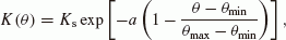  (14)
  

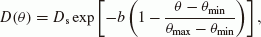  (15)

  where K_s is the saturated permeability, D_s is the saturated diffusivity, a and b are positive constants and θ_max and θ_min are the maximum and minimum water content, respectively. For Isawa Fan, the soil parameter values were taken to be

  

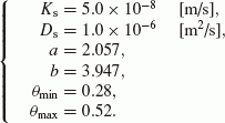  (16)

  K_s and θ_max were derived from tests on soil sampled near the gravity observatory (Klute and Dirksen, 1986; Grossman and Reinsch, 2002), whereas D_s, a, b and θ_min were estimated by trial-and-error fitting of the theoretical results to the observed moisture variation. Note that these soil parameter values are consistent with those for typical silt soil (Olsson and Rose, 1978; Amemiya et al., 1991; Nishigaki, 1991). We used these soil parameter values for the entire computational region, assuming homogeneous soil around the observatory.

With the water distribution, θ(z, t), estimated as above, the changes in gravity associated with variations in the water distribution below the ground surface, g_w(t), can be calculated by using the sum of the attraction effects (e.g., van Camp et al., 2006; Hasan et al., 2008):

(17)

(18)

where G is the gravitational constant, ρ_w is the water density, (x₀, y₀, z₀) is the position of the gravimeter and the constant 2πρ_wG (≃41.9 [µgal/m]) represents the attraction effect of a 1-m-thick infinite water plane. Note that in the Fortran code, Eq. (17) was reformulated as the simple summation of the moisture θ _i :

(19)

for an integer N satisfying NΔz = d. In the equations, topographic undulation and horizontal heterogeneity of the water distribution were disregarded, because the water distribution is thought to be horizontally homogeneous in flat areas like Isawa Fan as gravity changes are concerned.

In addition to g_w(t), we also denote the instrumental drift component and the gravity error as g_d(t) and e(t), respectively, in order to reproduce the observed gravity change, g_obs(t),as

(20)

The instrumental drift for superconducting gravimeters is accurately represented by the exponential attenuation function, as discussed by van Camp and Francis (2007). However, the reported attenuation time constants are estimated using data from a period of several years; hence, with only two years of observation data on Isawa Fan, estimating the attenuation time constant is difficult. Therefore, here we assumed a simple linear drift (Amalvict et al., 2001; Crossley et al., 2005):

(21)

where A_di and A′_di are the intercepts, and A_ds and A_ds are the drift rates. Note that different parameters are set before and after the exchange of the gravimeter’s controller. Since an arbitrary drift rate, −0.095 µgal/day was subtracted from the raw gravity data (see the previous section), the total drift rates are A_di − 0.095 (before 27 June, 2009) and A′_di − 0.095 (after 27 July, 2009). In this study, the least-squares method was applied to estimate the above four parameters, where the L₂ norm, , was minimized.

Hence, in the manner described, we estimated the soil moisture (θ(z, t)) and the gravity (g_w(t) and g_d(t))at Mizusawa during the three years from 2008 to 2010. In the next section, we compare the estimated results and the observed data (Fig. 3) during only two years, from January 2009 to December 2010, owing to preliminary computations suggesting that about half a year is required for the moisture distribution θ(z, t) to undergo a transition from the steady state to the unsteady state.

4. Modeled Results

The solid line in Fig. 4 shows the estimated distribution of steady-state soil moisture, θ_s(Z), with respect to the height from the water table, Z (Fig. 2). The estimated soil moisture is at its maximum at the water table (θ_s(0) = θ_max = 0. 52) and decreases gradually with the weakening capillary effect at the upper soil. The decreasing trend for 0 ≤ Z ≤ 3 [m] is linear rather than exponential, which is consistent with the steady-state water distribution of typical clay and silt (e.g., figure 9.4.5 in Bear, 1972; figure 3.15 in Jury and Horton, 2004). The soil moisture at over 5 m converges to 0.38, because water infiltration from the upper layer balances water diffusion from the lower layer. The convergence value, defined as θ _∞ , can be estimated as

(22)

which is derived from (see Eq. (4)) and the parameters in Eqs. (13) and (16). The steady-state soil moisture value at ground surface level during the two years, 0.5 ≤ Z ≤ 3 [m] (Fig. 3(d)), is 0.41 ∼ 0.50 and coincides with the observed moisture at Mizusawa (Fig. 3(c)). In these respects, the estimated distribution of θ_s(Z) is consistent with the soil characteristics and observations at Mizusawa. As explained in the previous section, this steady-state moisture distribution is used as the initial distribution of θ(z, t) (Eq. (12)). For the case of Mizusawa, we utilized the distribution at 0 ≤ Z ≤ 0.52 [m] for θ(z, 0), since the initial water level was located at 0.52 m below the ground surface (cf. y-intercept of Fig. 3(d)).

Fig. 4

Estimated steady-state profile of soil moisture, θ_s, at Isawa Fan, with respect to height from the water table, Z. Solid and gray lines are estimated profiles assuming full infiltration (p = 1.0) and no infiltration (p = 0.0) into the ground, respectively. Dashed line denotes ground level on 1 January 2008 (see y-intercept of Fig. 3(d)).

Figure 5 shows the estimated soil moisture change at a depth of 0–1 m below the ground surface, when assuming that all precipitation is infiltrated into the ground soil (i.e., p = 1.0). The moisture value at depths of 5–10 cm (Fig. 5(a)) increases considerably at precipitation events, and the value becomes saturated (θ = 0.52) during a heavy rainfall event in the latter half of April 2009. After each rainfall event, the moisture at 5–10 cm depths decreases exponentially, attributable to both evapotranspiration at the surface and soil water infiltration into the deeper layer. The estimated amplitude of the soil moisture variation during summer (April to October) is about 0.22 (0.30 ≤ θ ≤ 0.52), about 1.5 times larger than that during winter (November to March; 0.38 ≤ θ ≤ 0.52), and is due to more evapotranspiration occurring in summer (gray bar in Fig. 3(a)) making the uppermost soil drier than in winter.

Fig. 5

Estimated variation of soil moisture during 2 years from 2009 to 2010 with p = 1.0 at (a) 5–10 cm, (b) 15–20 cm, (c) 25–30 cm, (d) 35–40 cm, (e) 55–60 cm and (f) 95–100 cm below the ground surface. The vertical axis ranges from θ_min (= 0.28) to θ_max (= 0.52). (g) Average of the estimated soil moisture 0–1 m below the ground surface (solid line), with 1-σ error range of observed gravity (gray area) and observed daily precipitation (gray bar).

In contrast, the moisture response to precipitation at deeper layers (Fig. 5(b)–(f)) has greater attenuation and shows a larger lag because of soil moisture diffusion (Eq. (5)). For example, the estimated soil moisture increase from April to May 2010 is attenuated by a half at depths between 25–30 cm and by a quarter between 95–100 cm, and the time of the first moisture peak is delayed by 1.3 and 6.5 days, respectively. On occasion, a number of precipitation events concatenate into one moisture peak, as seen in April 2009, July 2009 and July 2010. Thus, non-linear characteristics in soil water equations can be seen; the proceeding infiltration fronts draw level with the initial front, since the initial infiltration increases soil moisture, θ; permeability, K(θ) (Eq. (14)), and diffusivity, D(θ) (Eq. (15)); and soil moisture speed, |υ| (Eq. (4)), in sequence (figure 2.17 after Nakano, 1991).

The solid line in Fig. 5(g) represents the average estimated soil moisture 0–1 m below the ground surface, θ(t). The average soil moisture changes between 0.37 and 0.50, and correlates to the observed soil moisture at Mizusawa to within one-sigma error range (gray area in Fig. 5(g)). It must be emphasized here that the use of adequate soil parameters (Eq. (16)) is essential for obtaining accurate water distributions in soil. Even though we equate snowfall to be equivalent to rainfall on the ground surface, the similar precision can be estimated for the moisture content even in winter. We attribute this result to less precipitation in winter resulting in small changes in soil moisture distribution, and most of the covering snow infiltrating as snowmelt water, even if there is a lag between snowfall and melting.

The black line in Fig. 6(a) shows the estimated gravity change associated with soil water and groundwater, g_w(t). It can be seen from this figure that g_w(t) increases steeply during precipitation events, and it changes a maximum of ∼8 µgal according to the precipitation amount at each event. After precipitation, g_w(t) decreases linearly as opposed to exponentially, because a linear function can be produced from the superposition of multiple exponential functions (such as θ(z, t)) having increasing time lags (Kazama and Okubo, 2009). In addition, the rate of gravity decay changes seasonally, principally because of the seasonal variation of evapotranspiration (Figs. 3(a) and (b)); for example, the rate of decay in August 2009 (∼ −6 [µgal/month]) is about one-quarter of that in January 2010.

Fig. 6

Gravity changes due to soil moisture distribution and instrumental drift, from 2009 to 2010. (a) Solid line and gray bar are soil moisture component, g_w(t), in the estimated gravity and observed daily precipitation, R(t), respectively. (b) Thin, gray and thick lines are estimated drift component, g_d(t), observed gravity, g_obs(t) and estimated total gravity, g_cal(t), respectively. On the right, values for estimated drift parameters (A_ds and A′_ds), root mean square (RMS) and correlation coefficient (CC).

The thin line in Fig. 6(b) plots the linear gravity change associated with the instrumental drift, g_d(t), calculated from the least-squares method. The slopes before and after the instrumental maintenance in June 2009 are −0.009 and −0.018 µgal/day, respectively. With −0.095 µgal/day already subtracted from the gravity data (see Section 2), the total drift rates are therefore −0.104 and −0.113 µgal/day, respectively.

The thick line in Fig. 6(b) shows the predicted total change in gravity, Although g_cal(t) qualitatively reproduces gravity increases during precipitation events, the amount of the increase for the calculated gravity is about twice that of the observed gravity (gray line), as seen in April 2009, July 2010 and September 2010. Additionally, the estimated gravity decay after each precipitation is faster than that observed, and the difference between g_obs(t) and g_cal(t) is larger than 3 µgal in August 2009 and April 2010.

To summarize these results: (1) Our model can reproduce the water distribution in soil within the observation error range (Fig. 5(g)) owing to the choosing of adequate soil parameters. (2) The estimated gravity value, g_cal(t) (Eqs. (17) and (20)), is not consistent with that observed, in terms of both the increased gravity amounts during precipitation and the rates of gravity decrease after precipitation. A potential cause of this inconsistency is the horizontal heterogeneity of the water distribution in the vicinity of the gravimeter; for the case of Mizusawa, the gravity observation building itself could affect the horizontal water heterogeneity, and the subsequent gravity disturbance (e.g., Creutzfeldt et al., 2010a). Thus, in the following subsection, an effect of the building will also be taken into account when estimating the water distribution and the gravity change.

4.1 Building effect

Assuming that precipitation does not infiltrate into the soil in the area of the observation building, the infiltration capacity, p, can be defined as

(23)

Furthermore, if the soil and water levels are continuous between the inside and outside of the building (Fig. 2), then two boundary conditions for estimating θ(z, t) below the building can be written as follows: (1) The vertical water flow velocity on the ground surface is zero; Å(z_s, t) = 0. (2) The soil below the water table is saturated; θ(z ≤ h(t), t) = θ_max. (See Eqs. (10) and (11) for outside the building.) Thus, the diffusion equation (Eq. (5)) is solved for the water distribution inside and outside the building (Fig. 5).

The gray line in Fig. 4 shows the steady-state distribution of the soil moisture for the ground inside the building, is a maximum and is saturated at the water table, and decreases at a faster rate than for the steady-state moisture distribution outside the building, θ_s(Z; p = 1) (the black line in Fig. 4). Moreover, θ_s(Z; p = 0) converges to a minimum value θ_min (= 0.28) at Z > 4 [m], since water is not supplied from the upper layers.

Figure 7(a)–(f) shows the estimated variation of soil moisture over time inside the building, θ(z, t; p = 0). Note that the steady-state moisture profile, θ_s(Z; p = 0) at 0 ≤ Z ≤ 0.52 [m], is utilized for the initial profile, θ(z, 0; p = 0) (Eq. (12)). θ(z, t; p = 0) does not respond to small precipitation events, such as θ(z, t; p = 1) (Fig. 5), but does change when the water level increases to a depth of 1.0 m below the ground surface (Fig. 7(g)), as seen in May, April, July 2009 and July 2010. The peak moisture at a depth of 5–10 cm (Fig. 7(a)) occurs later than that at 95–100 cm (Fig. 7(f)) by approximately half a month, because soil moisture diffuses from the water table only, not from the surface.

Fig. 7

Estimated variation of soil moisture during 2 years from 2009 to 2010 with p = 0.0 at (a) 5–10 cm, (b) 15–20 cm, (c) 25–30 cm, (d) 35–40 cm, (e) 55–60 cm and (f) 95–100 cm below the ground surface. The vertical axis ranges from θ_min (= 0.28) to θ_max (= 0.52). (g) Observed water level (solid line) and daily precipitation (gray bar). The horizontal dashed line indicates −1 m level from ground surface.

To accurately estimate the changes in gravity originating from soil moisture distributions, both θ(z, t; p = 1) and θ(z, t; p = 0) must be integrated with ratios according to the observation geometry. Defining the depth from the ground surface as ζ (= z_s − z; Fig. 2), the integration ratios at depth ζ for inside and outside the building can be written as

(24)

(25)

(26)

where δz is an arbitrary thickness of the water plane, and x₁, x₂, y₁ and y₂ are the edge positions of the observation building (Fig. 2). For the case of the Mizusawa Observatory, we used geometric parameters:

(27)

Figure 8 shows the calculated amplitude ratios, a_in(ζ) and a_out(ζ). The amplitude ratio for inside the building, a_in(ζ), reaches a maximum at surface level (∼0.71) and decreases with depth, because the region occupied by the observation building (25 × 16 [m²]) located at a deeper depth can be seen with a narrower viewing angle by the gravimeter. In addition, the two amplitude ratios are equal to 0.50 when ζ = 2.9 [m].

Fig. 8

Gravity amplitude ratio with respect to depth from the ground surface, ζ (Fig. 2). Dashed and solid lines represent the gravity attraction effect of soil water inside and outside the observation building—a_in(ζ) and a_out(ζ)—, respectively.

These amplitude ratios are employed in gravity estimation as follows:

(28)

(29)

(30)

Here, and are the attraction effect of soil moisture inside and outside the building, respectively. The two thin black lines in Fig. 9(a) depict the estimated and . The amplitudes of and are 2.8 and 2.6 µgal, respectively, which are 38% and 35% of the amplitude of the original estimated gravity, g_w(t) (gray line in Fig. 9(a)). The profile of the time variations is nearly the same for and ; however, the gravity response of is more sensitive to small precipitation events because the integrand of , θ(z, t; p = 1) (Fig. 5), increases significantly for small precipitation events when compared with θ(z, t; p = 0) (Fig. 7). The thick black line in Fig. 9(a) plots the total effect on the gravity due to the soil moisture, . The amplitude of is about 67% of that for g_w(t), showing that the observation building can reduce gravity responses to precipitation events by up to a third.

Fig. 9

Gravity change due to soil moisture distribution and instrumental drift from 2009 to 2010, considering building effects. (a) Top and middle lines are gravity changes due to soil moisture inside and outside the observation building ( and ), respectively. Lower thick and gray lines are total gravity change due to soil moisture with and without the building effect, (Eq. (28)) and g_w(t) (Eq. (17)), respectively. Gray bar is observed daily precipitation, R(t), at Mizusawa. (b) Thin, gray and solid lines are estimated drift component, g_d(t), observed gravity, g_obs(t), and estimated total gravity, g_cal(t), during 2 years from 2009 to 2010. On the right, values for A_ds and , RMS and CC. (c) Gray and solid lines are observed gravity, g_obs(t), and estimated total gravity, g_cal(t) during 50 days from 26 April to 15 June, 2010 (dashed square in Fig. 9(c)). Gray bar is observed hourly precipitation, R(t), at Mizusawa. On the right, values for , RMS and CC.

In Fig. 9(b) and (c), the estimated gravity, g_cal(t), composed of the moisture effect and the drift effect (Eq. (28)) is compared with the observed gravity, g_obs(t). Figure 9(c) shows gravity changes for 50 days (from 26 April to 15 June, 2010). The amplitude of g_cal(t) during these 50 days is ∼3.8 µgal, comparable with that of g_obs(t) (4.4 µgal). Variations of g_cal(t) over this period are also consistent with g_obs(t), both in gravity increases during each precipitation event and in peak-time delays, which are about 3–4 days after the beginning of each event. This peak-time delay in gravity is most likely a consequence of the delay in the water level increase around the gravimeter, since the unconfined groundwater must flow from the upper part of Isawa Fan to Mizusawa Observatory (cf. detailed discussion in Section 5.2). The hydrological model presented here can reproduce the delayed gravity response to precipitation, because the observed water level, h(t), is utilized as one of the boundary conditions when estimating the moisture distributions. In addition, g_cal(t) is consistent with g_obs(t) for gravity reduction rates after precipitation, originating from the instrumental drift ( [µgal/day]) and water mass loss in the soil owing to evapotranspiration and groundwater flow. Hence, in the above respects, the hydrological model reproduced the observed gravity changes during the 50 days both qualitatively and quantitatively, with a small RMS (0.44 µgal) and a high correlation coefficient (CC: 0.89).

Conversely, the variation of over a longer period is in part contradictory with g_obs(t). The gray and thick black lines in Fig. 9(b) show the observed and estimated changes in gravity (g_obs(t) and g_cal(t)), respectively. When compared with (the thick black line in Fig. 6(b)), the increase in amplitude of g_cal(t) during each precipitation event agrees with g_obs(t), especially in April 2009, October 2009 and January 2010. In addition, the RMS and CC values in Fig. 9(b) show that there is better agreement between g_cal(t) and g_obs(t) than equivalent values resulting from Fig. 6(b), suggesting the significance of considering the building effect in estimating accurate gravity changes. However, g_cal(t) still differs from g_obs(t) by up to 4 µgal, as seen in July 2009, March–May 2010 and July–August 2010. The gravity difference, , seems to be positive in summer (June–August) and negative in winter and spring (February–May), implying the existence of an annual gravity signal in g_obs(t). (Note that the negative gravity difference in winter 2009 might be compensated for by the large decreasing trend, A_ds = −0.026 [µgal/day].)

To summarize the results in this section: (1) The hydrological model that considers building effects can reproduce the observed gravity change at Mizusawa during a 50-day period with an accuracy of about 0.4 µgal (Fig. 9(c)). (2) The variation over the two years for the estimated gravity is not still consistent with observed annual gravity changes. The latter might be caused by the land-water scale covered in the hydrological model; since the model uses the locally-observed water level and precipitation in the boundary conditions, only local moisture distributions and their consequent short-period (∼50 days) gravity changes are accurately predicted. In contrast, the model proposed here does not take into account the regional/global horizontal water distribution, and therefore cannot reproduce long-period (∼2 years) changes in gravity, including the annual component of the gravity. Although, in principle, two- or three-dimensional land-water modeling (e.g., Kazama and Okubo, 2009) is required to address the highlighted concern, this study focuses on a simple hydrological model to estimate accurate land-water distributions and gravity changes, as indicated in Introduction. Thus, in the next section, the amplitude of the annual change in gravity will be calculated by using the least-squares method. Furthermore, the effects resulting from a covering of snow will be considered to estimate more accurate changes in gravity in winter, because, compared with rain, snow remaining on the ground and building roofs can cause a significant gravity change over a longer duration.

4.2 Annual gravity change and snow effect

Here, the annual gravity change, g_a(t), and the snow-covering effect, g_s(t), are incorporated into g_cal(t):

(31)

where g_a(t) and g_s(t) are defined as

(32)

(33)

for T = 365 [day], and snow depth at Isawa Fan, S(t) (gray bar in Fig. 3(b)). In these equations, we assume a simple periodic function for g_a(t), and a simple proportional relationship between g_s(t) and S(t). Note that, in our hydrological model, we ignored effects from snow sublimation at the top of the covered snow and from the interaction between accumulated snow and soil water, owing to the physical mechanisms of these effects currently not being fully understood (e.g., Pomeroy et al., 2007; Strasser et al., 2008). The three coefficients (A_ac, A_as and A_s) are calculated by the least-squares method, in addition to the instrumental drift parameters (A_di, A_ds, and ) in g_d(t) (Eq. (21)).

The central line in Fig. 10(a) plots g_a(t). The estimated amplitudes for the cosine and sine functions are 0.86 and 1.16 µgal, respectively, and the total annual amplitude is

(34)

g_a(t) attains its maximum value on 24 February (day of year: 55) and its minimum value on 25 August (day of year: 237). This annual gravity change may be due to vertical land surface deformation from water and atmospheric loads (e.g., Sato et al., 2001; Boy et al., 2002; Llubes et al., 2004). For example, Heki (2004) modeled load deformations resulting from snow, the atmosphere, soil moisture, fresh water impoundment and seawater, and found that a combination of these mass loads can subside the land surface in northern Japan by about 1 cm in winter (figure 16 in Heki, 2004). Gravity changes resulting from ground surface height modifications can be written as

(35)

where ρ _r and Δh are the rock density and the surface height change (in mm), respectively. If typical values for rock density (ρ_r= 2.67 [g/cm³]) and an assumed surface height change (Δh = −10 [mm]) are substituted into this equation, the change in gravity is found to be Δg = 1.97 [µgal]. Accordingly, the loading effect can explain about two-thirds of the estimated annual gravity change peak-to-peak (2.90 µgal). Conversely, ∼1 µgal of annual gravity changes are still unexplained and, as touched upon in the last part of this section, hydrological modeling in higher dimensions may reproduce the observed gravity more accurately.

Fig. 10

Gravity changes due to soil moisture, instrumental drift, regional/global water distributions and snow from 2009 to 2010. (a) Three lines: (top) soil moisture effect, , (middle) annual gravity change, g_a(t), and (bottom) snow effect, g_s(t). (b) Dashed line is estimated instrumental drift, g_d(t), and thin solid line is sum of g_d(t), ga(t) and g_s(t). Gray and thick solid lines are observed gravity, g_obs(t), and estimated total gravity, g_cal(t), respectively. Gray bar is observed daily precipitation, R(t), at Mizusawa. On the right, values for A_ds, , A_ac, A_as and A_s, RMS and CC.

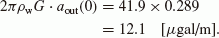
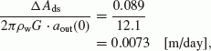
The lower solid plot in Fig. 10(a) is the estimated snow effect, g_s(t). g_s(t) decreases during the snow-covering season, since the estimated proportionality factor, As, is less than zero (−0.084 µgal/cm). This gravity decrease is, in particular, attributable to the attraction effect of covering snow on the building roof. When snow is accumulated on the ground and the roof to a depth of Δhs, the gravity attraction due to the snow is

(36)

where ρ_s and z_r are the snow density and the roof elevation (Fig. 2), respectively. Although the snow density varies depending on the exact place and the month of the year, the average snow density in northern Japan has been observed as 0.2 ≤ ρ_s ≤ 0.5 [g/cm³] (figure 4 in Heki, 2004). Moreover, if the average roof height is set as z_r − z₀ = 3 [m], the difference term (a_out − a_in) becomes negative:

(37)

showing that the snow attraction on the roof is greater than that on the ground for Mizusawa Observatory. Finally, the gravity attraction for 1-cm snow (Δhs = 10 [mm]) can be calculated as

(38)

which is consistent with the estimated proportionality factor, A_s = −0.084 [µgal/cm].

The thick line in Fig. 10(b) shows the g_cal(t), including the effects of soil moisture , the instrumental drift (g_d(t)), the annual gravity change (g_a(t)) and the covering snow (g_s(t)). Note that the instrumental drift rates are A_ds − 0.095 = −0.108 [µgal/day] (before June 2009) and [µgal/day] (after June 2009), because −0.095 µgal/day was already subtracted from the original gravity data (see Section 2). It can be seen that g_cal(t), including the annual term, matches g_obs(t) (gray line) more closely, especially for August 2009, March–May 2010 and July–August 2010, when compared with the thick line in Fig. 9(b) (not including the annual gravity term). g_cal(t) also agrees with g_obs(t) during winter (such as in February 2009 and January 2010), owing to the snow-covering effect applied in the model. In addition, the RMS and the CC values are 1.03 µgal and 0.97, respectively, showing a good correlation between g_obs(t) and g_cal(t). From these results, it can be seen that, by adding both the annual gravity term and the snow effects (Eq. (31)), our proposed hydrological modeling can now reproduce long-term gravity changes within about 1 µgal RMS.

In contrast, a large discrepancy remains between g_obs(t) and g_cal(t) of about 2 µgal in March 2009, August–September 2009 and April 2010. The cause of this discrepancy may lie in the low dimension of the hydrological modeling; here, we have supposed a simple vertical soil water flow (Eq. (5)) and two- or three-dimensional modeling of the water flow (e.g., Kazama and Okubo, 2009) would match the observed gravity including the annual component, with a higher accuracy. Moreover, to precisely predict gravity changes in winter, snow physics must be added into our hydrological model, such as water interaction between covering snow and soil water (Pomeroy et al., 2007), water sublimation at the top of the covering snow (Strasser et al., 2008), and spatiotemporal heterogeneity of the snow depth and the density (Heki, 2004; Doi et al., 2010).

5. Discussion

5.1 Dependency on soil parameters

The hydrological model requires parameters predominantly related to soil physics, for example, P₀ (Eq. (13)), K_s, D_s, a, b, θ_min, θ_max (Eq. (16)) and p (Eq. (23)). Therefore, estimated results (e.g., moisture θ(z t) and gravity g_cal(t)) will change according to the parameter values that are used in the model. Figures 11–15 show the dependencies of moisture and gravity on the parameters K_s, D_s, a, b and P₀. In each figure, moisture and gravity variations are shown for five different parameter values as (1)–(5), with the default parameter value (Eqs. (13) and (16)) corresponding to (3).

Fig. 11

Dependency of soil moisture distributions and gravity changes on saturated permeability, K_s. For K_s equal to (1) 2.0 × 10⁻⁸, (2) 3.0 × 10⁻⁸, (3) 5.0 × 10⁻⁸ (default value: thick line), (4) 7.0 × 10⁻⁸, (5) 1.0 × 10⁻⁷ [m/s]. (a) Steady-state soil moisture profile with p = 1.0, θ_s(Z; p = 1). (b) Time variation of soil moisture at 50 cm below the ground surface with p = 1.0, θ(z_s − 0.5, t; p = 1). (c) Gravity changes due to soil moisture distribution, g_w(t).

The upper panel (a) in each figure shows the steady-state moisture distribution for p = 1.0; θ_s(Z; p = 1). The steady-state moisture depends on the model parameters in the following two respects. First, the asymptotic value, θ_∞, changes when K_s, a or P₀ is changed (Figs. 11(a), 13(a) and 15(a)). As seen in Eq. (22), θ_∞ has a positive correlation with a and P₀, and is negatively correlated to K_s. Second, the asymptotic rate becomes lower if D_s is greater (Fig. 12(a)) or b is smaller (Fig. 14(a)). This reduction is because the unsaturated diffusivity D(θ) (Eq. (15)) increases and the capillary effect from the water table is stronger, with larger D_s or smaller b.

Fig. 12

Dependency of soil moisture distributions and gravity changes on saturated diffusivity, D_s.For D_s equal to (1) 1.0 × 10⁻⁷, (2) 3.0 × 10⁻⁷, (3) 1.0 × 10⁻⁶ (default value: thick line), (4) 3.0 × 10⁻⁶, (5) 1.0 × 10⁻⁵ [m²/s]. (a) Steady-state soil moisture profile with p = 1.0, θ_s(Z; p = 1). (b) Time variation of soil moisture at 50 cm below the ground surface with p = 1.0, θ(z_s − 0.5 t; p = 1). (c) Gravity changes due to soil moisture distribution, g_w(t).

Fig. 13

Dependency of soil moisture distributions and gravity changes on a. For a equal to (1) 1.000, (2) 1.500, (3) 2.057 (default value: thick line), (4) 3.000, (5) 5.000. (a) Steady-state soil moisture profile with p = 1.0, θ_s(Z; p = 1). (b) Time variation of soil moisture at 50 cm below the ground surface with p = 1.0, θ(z_s − 0.5, t; p = 1). (c) Gravity changes due to soil moisture distribution, g_w(t).

Fig. 14

Dependency of soil moisture distributions and gravity changes on b. For b equal to (1) 0.000, (2) 2.000, (3) 3.947 (default value: thick line), (4) 6.000, (5) 8.000. (a) Steady-state soil moisture profile with p = 1.0, θ_s(Z; p = 1). (b) Time variation of soil moisture at 50 cm below the ground surface with p = 1.0, θ(z_s − 0.5 t; p = 1). (c) Gravity changes due to soil moisture distribution, g_w(t).

Fig. 15

Dependency of soil moisture distributions and gravity changes on averaged effective precipitation, P₀. For P₀ equal to (1) 5.0 × 10⁻⁹, (2) 1.0 × 10⁻⁸, (3) 1.5 × 10⁻⁸ (default value: thick line), (4) 2.0 × 10⁻⁸, (5) 3.0 × 10⁻⁸ [m/s]. (a) Steady-state soil moisture profile with p = 1.0, θ_s(Z; p = 1). (b) Time variation of soil moisture at 50 cm below the ground surface with p = 1.0, θ(z_s − 0.5, t; p = 1). (c) Gravity changes due to soil moisture distribution, g_w(t). Note that estimated time variations match exactly for all precipitation values, and the plots overlap in (b) and (c).

The central panel (b) in Figs. 11–15 shows the variation of the moisture over time at 50 cm below the ground surface for p = 1.0; θ(z_s − 0.5, t; p = 1). The moisture does not change even if the value of P₀ is changed (Fig. 15(b)), since P₀ relates only to the steady-state moisture profile, and not to the time-variable moisture, and the contribution from the difference in the steady-state moisture profiles (Fig. 15(a)) is small for the time-variable moisture; the steady-state profiles up to only 52 cm are utilized for the initial moisture distribution for the case of Isawa Fan (see beginning of Section 4). In addition, the moisture changes are slight (0.02 at most) when the values of a and b are altered (Figs. 13(b) and 14(b)), implying that the effect of soil parameter non-linearity (Eqs. (14) and (15)) is small when estimating the time-dependent moisture for the case of Mizusawa. Conversely, θ(z_s − 0.5, t; p = 1) changes considerably for changes in K_s or D_s (Figs. 11(b) and 12(b)). For example, when K_s is varied from 5.0 × 10⁻⁸ down to 3.0 × 10⁻⁸ and up to 7.0 × 10⁻⁸ [m/s], the moisture value increases and reduces by ∼0.04, respectively (Fig. 11(b)). Furthermore, when D_s is changed from 1.0 × 10⁻⁶ down to 3.0 × 10⁻⁷ and up to 3.0 × 10⁻⁶ [m²/s], the moisture value falls by about 0.08 and rises by about 0.07, respectively (Fig. 12(b)). These characteristics are mainly due to variations in K_s and D_s giving rise to changes in the soil water velocity v (Eq. (4)), and a balance change between the diffusion (the first term on the right-hand side of Eq. (5)) and the infiltration (the second term on the right-hand side of Eq. (5)) (e.g., Jury and Horton, 2004).

The lower panel (c) in Figs. 11–15 shows the gravity change, g_w(t) (Eq. (17)). Since g_w(t) is calculated from the integration of the moisture distribution, θ(z, t), the gravity dependence on each parameter is approximately equal to that of the moisture (Figs. 11(b)–15(b)). For example, the gravity amplitude sensitively changes according to variations in K_s and D_s by about 2.5 and 4 µgal, respectively. Moreover, the gravity difference is within 1 µgal for the changes in a (Fig. 13(c)) and b (Fig. 14(c)), and is exactly zero for changes of P₀ (Fig. 15(c)).

Thus, moisture and gravity variations are dependent on the soil parameter values, especially K_s and D_s for the case of Mizusawa presented here. That is, appropriate values for the soil parameters are essential for the realistic estimation of the moisture variation and the consequent gravity changes by the hydrological model. As described in Section 3, the soil parameter values in this study were derived from soil tests and the curve fitting to the observed moisture variation. Therefore, our hydrological model technique can be applied to any gravity stations, if reasonable parameter values are determined through observations of the soil parameters themselves and spatiotemporal moisture distributions.

5.2 Comparison between the physical model and empirical models

A number of researchers have predicted changes in gravity due to variations in land-water distributions through empirical models, by assuming a simple gravity response to the water plane thickness (e.g., Imanishi et al., 2006; Nawa et al., 2009). However, water flow is governed by nonlinear equations (Eq. (5)), and there are limitations to applying linearity theory to gravity responses (e.g., Kazama et al., 2005). Here, the results from three empirical gravity models are compared with those from our physical modeling. We now assume that gravity responds proportionally to the unconfined water level, h(t), the observed precipitation, R_tot(t), or the effective precipitation, P_tot(t), as follows:

(39)

(40)

(41)

(42)

In these equations, factors A _i (i = 1, 2, 3), A_di and A_ds are estimated by the least-squares method, so as to fit the observed gravity, g_obs(t), and each empirical gravity g _i (t) between 26 April and 15 June, 2010 (the same time period as in Fig. 9(c)). The black lines in Fig. 16 are the calculated empirical gravities, and we can infer the following from these plots:

• The proportional coefficient between the water level and the gravity is A₁ = 1.68 [µgal/m] (Fig. 16(a)). This value may be interpreted as the soil moisture in the unsaturated layer increased by about 4 volumetric % in an infinite half-space, assuming constant moisture values in the saturated and unsaturated layers (θ_sat and θ_unsat, respectively) as follows:

  

  (43)
  

  (44)

  (θ_sat − θ_unsat) is close to the observed moisture increase during precipitation events (Fig. 3(c)), though this model makes too many simplifying assumptions for the hydrological structure in soil. (The actual moisture value in the unsaturated layer is not constant, but increases in the lowermost part of the unsaturated layer owing to the capillary effect, as shown in Fig. 4.)

• The black lines in Figs. 16(b)–(c) show the empirical gravity models, g₂(t) and g₃(t). The proportional coefficients between the precipitations in the empirical models and the gravity are 28.4 and 25.3 µgal, respectively, both about twice as large as the expected instant gravity response for a 1-m precipitation outside the observation building,

  

  (45)

  This deviation might be a result of precipitation on the building infiltrating into the ground outside of the building through the guttering downpipes, suggesting the necessity for consideration of a horizontally heterogeneous precipitation (i.e., P = P(x, y, t)) in our hydrological model. Another reason could be that the observed gravity, g_obs(t) (gray line in Figs. 16(a)–(c)), cannot be fully explained by an instant response to precipitation, such as R(t) and P(t), because g_obs(t) is highly dominated by the water level change, h(t), for the case of Mizusawa (as demonstrated later).

• The difference in the gravity reduction rate (A_ds) between g₂(t) and g₃(t) is

  

  (46)

  This rate difference is exactly derived from the evapotranspiration, because the evapotranspiration effect is included in the second term in Eq. (40) and in the first term in Eq. (41). Therefore, the mass loss rate converted from Δ A_ds is

  

  (47)

  which is approximately equal to the evapotranspiration rate in summer (gray bar in Fig. 3(a)).

• A further point of interest is in the increase timings of the calculated gravity during precipitation events. Although g₂(t) and g₃(t) increase sharply in synchronization with precipitation (Fig. 16(d)), the timing of these increases is about 1 day earlier than for the observed gravity. In contrast, the gravity g₁(t) is consistent with the observed gravity, even for the increase timings, since g₁(t) is estimated from the water level change, h(t), whose peak time is delayed due to horizontal groundwater flow from the upper part of Isawa Fan. These facts suggest that, in the case of Isawa Fan, the primary source of the observed gravity is water level changes in the saturated layer, rather than instant mass increase near the ground surface from precipitation. (Our proposed hydrological model can also reproduce the peak-time delay of the observed gravity, as shown in Fig. 9(c), because the water level data is employed in one of the boundary conditions.)

Fig. 16

Gravity changes from empirical models. (a) Gray and solid lines are observed gravity, g_obs(t), and estimated gravity, g₁(t), from an empirical model assuming a linear response to water level change, h(t). (b) Gray and solid lines are observed gravity, g_obs(t), and estimated gravity, g₂(t), from an empirical model assuming a linear response to precipitation, R_tot(t). (c) Gray and solid lines are observed gravity, g_obs(t), and estimated gravity, g₃(t), from an empirical model assuming a linear response to effective precipitation, P_tot(t). On the right of the figures, values for A₁, A₂, A₃ and Ads, RMS and CC. (d) Gray bar and solid line are observed hourly precipitation, R(t), and cumulative precipitation, R_tot(t), respectively.

From the above, the empirical models can reproduce the observed gravity in rapid increases during precipitation and gradual decreases after precipitation, with smaller RMS values and larger CCs (right side of Figs. 16(a)–(c)) than those of our hydrological modeling (right side of Fig. 10(b)). However, the empirical models only fit the observed gravity with arbitrary functions; they do not account for the non-linear flow of the soil moisture. As described in Introduction, the hydrological gravity changes should be modeled and corrected independently of the observed gravity data, since the empirical models mostly tend to even subtract the solid-earth gravity signal from the observed gravity. Therefore, we emphasize that the physical hydrology model presented here is important for generating realistic water distributions and estimating the consequent changes in gravity.

6. Conclusions

We gathered hydrological, meteorological and superconducting gravity data at Isawa Fan in northern Japan, and modeled the spatiotemporal soil moisture distribution and the resultant gravity changes by using hydrological equations. In the hydrological modeling, the Richards equation is numerically solved for soil moisture θ(z, t), and spatial integration of θ(z, t) is performed, in order to calculate changes in gravity due to soil moisture. Estimated θ(z, t) values are consistent with those observed at Isawa Fan within the limits of observation error. When adequate soil parameters and building effects are included in the model, the estimated gravity g_cal(t) (Eq. (28)) agrees with the observed superconducting gravity g_obs(t) during a 50-day period within 0.4 µgal RMS. However, over a longer period (∼2 years), g_cal(t) cannot fully reproduce observed annual gravity changes, because the proposed model only considered variations in the local water distribution and the associated short-period (∼50 days) gravity change. Although, in principle, high-dimensional physical modeling must be applied to a larger region including Isawa Fan (e.g., Kazama and Okubo, 2009), here we added two effects— annual gravity change and snowfall—into g_cal(t), and calculated proportionality coefficients (A_ac, A_as and A_s)by the least-squares method. The reformulated gravity equation (Eq. (31)) matched the observed gravity g_obs(t), including the annual gravity change, with a low RMS value (∼1.0 µgal) and high CC (0.97). The calculated amplitudes of the annual gravity (∼1.5 µgal) and snowfall effect (∼ −0.08 µgal/cm) can be explained by water mass loading (Heki, 2004) and snow accumulation on the ground and the building roof, respectively.

Finally, we remark that gravity corrections for hydrological effects by physical models are essential for accurately detecting the mass transfers associated with earthquakes and volcanoes from gravity data. Our physical modeling can be utilized for hydrological gravity corrections at all gravity stations in plain areas, if sufficient soil parameter values and certain observation data (e.g., precipitation and water level) are available. In the future, we will release the Fortran coding used for this hydrological modeling as the “G-water 1D” program package, which will again be applied to the superconducting gravity data at Mizusawa in order to monitor the post-seismic gravity changes associated with the 2011 M_w 9. 0 Tohoku Earthquake (Ide et al., 2011;Ozawa et al., 2011).

References

Abe, M., S. Takemoto, Y. Fukuda, T. Higashi, Y. Imanishi, S. Iwano, S. Ogasawara, Y. Kobayashi, S. Dwipa, and D. S. Kusuma, Hydrological effects on the superconducting gravimeter observation in Bandung, J. Geodyn., 41, 288–295, 2006.
Aki, K. and P. Richards, Quantitative Seismology: Theory and Methods, 932 pp., W. H. Freeman, NY, 1980.
Amalvict, M., J. Hinderer, J.-P. Boy, and P. Gegout, A three year comparison between a superconducting gravimeter (GWR C026) and an absolute gravimeter (FG5#206) in Strasbourg (France), J. Geod. Soc. Jpn., 47, 334–340, 2001.
Amemiya, Y., S. Yabashi, T. Kondo, K. Nakayama, M. Kim, and S. Takahashi, Soil water diffusivity and unsaturated hydraulic conductivity of the volcanic soil under cold climate in northeastern Hokkaido, Tech. Bull. Fac. Hort. Chiba Univ., 44, 219–223, 1991 (in Japanese with English abstract).
Bear, J., Dynamics of Fluids in Porous Media, 764 pp., Elsevier, Netherlands, 1972.
Becker, J. J., D. T. Sandwell, W. H. F. Smith, J. Braud, B. Binder, J. Depner, D. Fabre, J. Factor, S. Ingalls, S.-H. Kim, R. Ladner, K. Marks, S. Nelson, A. Pharaoh, R. Trimmer, J. Von Rosenberg, G. Wallace, and P. Weatherall, Global bathymetry and elevation data at 30 arc seconds resolution: SRTM30.PLUS, Mar. Geod., 32, 355–371, 2009.
Betts, A. K. and J. H. Ball, Albedo over the boreal forest, J. Geophys. Res., 102(D24), 28901–28909, 1997.
Bower, D. R. and N. Courtier, Precipitation effects on gravity measurements at the Canadian absolute gravity site, Phys. Earth Planet. Inter., 106, 353–369, 1998.
Boy, J.-P. and J. Hinderer, Study of the seasonal gravity signal in superconducting gravimeter data, J. Geodyn., 41, 227–233, 2006.
Boy, J.-P., P. Gegout, and J. Hinderer, Reduction of surface gravity data from global atmospheric pressure loading, Geophys. J. Int., 149, 534–545, 2002.
Creutzfeldt, B., A. Guntner, H. Wziontek, and B. Merz, Reducing local hydrology from high-precision gravity measurements: a lysimeter-based approach, Geophys. J. Int., 183, 178–187, 2010a.
Christiansen, L., P. Binning, D. Rosbjerg, O. B. Andersen, and P. Bauer-Gottwein, Using time-lapse gravity for groundwater model calibration: An application to alluvial aquifer storage, Water Resour. Res., 47, W06503, 2011.
Creutzfeldt, B., A. Güntner, H. Thoss, B. Merz, and H. Wziontek, Measuring the effect of local water storage changes on in situ gravity observations: Case study of the Geodetic Observatory Wettzell, Germany, Water Resour. Res., 46, W08531, 2010b.
Crossley, D., J. Hinderer, G. Casula, O. Francis, H.-T. Hsu, Y. Imanishi, G. Jentzsch, J. Kaarianen, J. Merriam, B. Meurers, J. Neumeyer, B. Richter, K. Shibuya, T. Sato, and T. Van Dam, Network of super-conducting gravimeters benefits a number of disciplines, Eos Trans. AGU, 80, 121–126, 1999.
Crossley, D., J. Hinderer, and J.-P. Boy, Time variation of the European gravity field from superconducting gravimeters, Geophys. J. Int., 161, 257–264, 2005.
Davidson, J. M., L. R. Stone, D. R. Nielsen, and M. E. Larue, Field measurement and use of soil-water properties, Water Resour. Res., 5, 1312–1321, 1969.
Doi, K., K. Shibuya, Y. Aoyama, H. Ikeda, and Y. Fukuda, Observed gravity change at Syowa Station induced by Antarctic ice sheet mass change, 557–562, in Gravity, Geoid and Earth Observation, edited by S. P. Mertikas, 701 pp., IAG Symposia 135, Springer, Germany, 2010.
Francis, O., M. Van Camp, T. Van Dam, R. Warnant, and M. Hendrichx, Indication of the uplift of the Ardenne in long-term gravity variations in Membach (Belgium), Geophys. J. Int., 158, 346–352, 2004.
Furuya, M., S. Okubo, W. Sun, Y. Tanaka, J. Oikawa, H. Watanabe, and T. Maekawa, Spatiotemporal gravity changes at Miyakejima Volcano, Japan: Caldera collapse, explosive eruptions and magma movement, J. Geophys. Res., 108(B4), 2219, 2003.
Gardner, W. R. and M. S. Mayhugh, Solutions and tests of the diffusion equation for the movement of water in soil, Soil Sci. Soc. Am. Proc., 22, 197–201, 1958.
Goodkind, J. M., The superconducting gravimeter, Rev. Sci. Instrum., 70, 4131–4152, 1999.
Grossman, R. B. and T. G. Reinsch, Bulk density and linear extensibility, 201–228, in Methods of Soil Analysis, Part 4: Physical Methods, edited by J. Dane and G. Topp, 866 pp., Soil Sci. Soc. Am., Madison, Wis, 2002.
Hanada, H., T. Tsubokawa, and T. Suzuki, Seasonal variations of ground water level and related gravity changes at Mizusawa, Technical Reports of the Mizusawa Kansoku Center, National Astronomical Observatory, 2, 83–93, 1990 (in Japanese).
Harnisch, G. and M. Harnisch, Hydrological influences in long gravimetric data series, J. Geodyn., 41, 276–287, 2006.
Hasan, S., P. A. Troch, J. Boll, and C. Kroner, Modeling of hydrological effect on local gravity at Moxa, Germany, J. Hydrometeorol., 7, 346–354, 2006.
Hasan, S., P. A. Troch, P. W. Bogaart, and C. Kroner, Evaluating catchment-scale hydrological modeling by means of terrestrial gravity observations, Water Resour. Res., 44, W08416, 2008.
Heki, K., Dense GPS array as a new sensor of seasonal changes of surface loads, 177–196, in The State of the Planet: Frontiers and Challenges in Geophysics, edited by R. S. J. Sparks and C. J. Hawkesworth, Geophys. Monograph, 150, 410 pp, AGU, Washington, 2004.
Ide, S., A. Baltay, and G. C. Beroza, Shallow dynamic overshoot and energetic deep rupture in the 2011 Mw 9.0 Tohoku-Oki Earthquake, Science, 332, 1426–1429, 2011.
Idso, S. B., R. D. Jackson, R. J. Reginano, B. A. Kimball, and F. S. Nakayama, The dependence of bare soil albedo on soil water content, J. Appl. Meteor., 14, 109–113, 1975.
Iinuma, T., M. Ohzono, Y. Ohta, S. Miura, M. Kasahara, H. Takahashi, T. Sagiya, T. Matsushima, S. Nakao, S. Ueki, K. Tachibana, T. Sato, H. Tsushima, K. Takatsuka, T. Yamaguchi, M. Ichiyanagi, M. Takada, K. Ozawa, M. Fukuda, Y. Asahi, M. Nakamoto, Y. Yamashita, and N. Umino, Aseismic slow slip on an inland active fault triggered by a nearby shallow event, the 2008 Iwate-Miyagi Nairiku earthquake (Mw6.8), Geophys. Res. Lett., 36, L20308, 2009.
Imanishi, Y., T. Sato, T. Higashi, W. Sun, and S. Okubo, A network of superconducting gravimeters detects submicrogal coseismic gravity changes, Science, 306, 476–478, 2004.
Imanishi, Y., K. Kokubo, and H. Tatehata, Effect of underground water on gravity observation at Matsushiro, Japan, J. Geodyn., 41, 221–226, 2006.
Iwate Prefecture, Observation Information of Snowfall in Iwate Prefecture, http://www.josetu.jp/iwate/public/snowobs.aspx, 30 April 2011.
Jahr, T., G. Jentzsch, and A. Weise, Natural and man-made induced hydrological signals, detected by high resolution tilt observations at the Geodynamic Observatory Moxa/Germany, J. Geodyn., 48, 126–131, 2009.
Japan Meteorological Agency, Meteorological Statistics Information: Searching Past Meteorological Data, http://www.data.jma.go.jp/obd/stats/etrn/index.php, 17 May 2011.
Jury, W. A. and R. Horton, Soil Physics (6th ed.), 370 pp., Wiley, NJ, 2004.
Kazama, T. and S. Okubo, Hydrological modeling of groundwater disturbances to observed gravity: Theory and application to Asama Volcano, Central Japan, J. Geophys. Res., 114, B08402, 2009.
Kazama, T., S. Okubo, W. Sun, S. Matsumoto, and E. Koyama, Tracing magma head in the volcano with continuous gravity monitoring (2), Abstracts of Japan Earth and Planetary Science Joint Meeting 2005 CD-ROM], V055-006, Japan Geosci. Union, Tokyo, Japan, 2005.
Klute, A. and C. Dirksen, Hydraulic conductivity and diffusivity: Laboratory methods, 687–734, in Methods of Soil Analysis, Part 1: Physical and Mineralogical Methods, edited by A. Klute, 1358 pp., Soil Sci. Soc. Am., Madison, Wis, 19
Krause, P., M. Naujoks, M. Fink, and C. Kroner, The impact of soil moisture changes on gravity residuals obtained with a superconducting gravimeter, J. Hydrol., 373, 151–163, 2009.
Lampitelli, C. and O. Francis, Hydrological effects on gravity and correlations between gravitational variations and level of the Alzette River at the station of Walferdange, Luxembourg, J. Geodyn., 49, 31–38, 2010.
Leirião, S., X. He, L. Christiansen, O. B. Andersen, and P. Bauer-Gottwein, Calculation of the temporal gravity variation from spatially variable water storage change in soils and aquifers, J. Hydrol., 365, 302–309, 2009.
Llubes, M., N. Florsch, J. Hinderer, L. Longuevergne, and M. Amalvict, Local hydrology, the Global Geodynamics Project and CHAMP/GRACE perspective: Some case studies, J. Geodyn., 38, 355–374, 2004.
Longuevergne, L., J.-P. Boy, N. Florsch, D. Viville, G. Ferhat, P. Ulrich, B. Luck, and J. Hinderer, Local and global hydrological contributions to gravity variations observed in Strasbourg, J. Geodyn., 48, 189–194, 2009.
Meurers, B., M. Van Camp, and T. Petermans, Correcting superconducting gravity time-series using rainfall modelling at the Vienna and Membach stations and application to Earth tide analysis, J. Geod., 81, 703–712, 2007.
Miller, J. D. and G. J. Gaskin, ThetaProbe ML2x: Principles of operation and applications, MLURI Technical Note (2nd ed), 1–20, 1999.
Miura, T. and R. Okuno, Detailed description of calculation of potential evapotranspiration using the Penman equation, Trans. JSIDRE, 164, 157–163, 1993 (in Japanese with English abstract).
Murai, H. and Y. Iwasaki, Studies on function of water and soil conservation based on forest land (I): Influence of difference in forest condition upon water run-off, infiltration and soil erosion, Bull. Gov. For. Exp. Sta., 274, 23–84, 1975 (in Japanese with English abstract).
Nakano, M., Science of Mass Flow in Soils, 187 pp., University of Tokyo Press, Tokyo, 1991 (in Japanese).
Naujoks, M., C. Kroner, A. Weise, T. Jahr, P. Krause, and S. Eisner, Evaluating local hydrological modelling by temporal gravity observations and a gravimetric three-dimensional model, Geophys. J. Int., 182, 233–249, 2010.
Nawa, K., N. Suda, I. Yamada, R. Miyajima, and S. Okubo, Coseismic change and precipitation effect in temporal gravity variation at Inuyama, Japan: A case of the 2004 off the Kii peninsula earthquakes observed with a superconducting gravimeter, J. Geodyn., 48, 1–5, 2009.
Neumeyer, J., F. Barthelmes, O. Dierks, F. Flechtner, M. Harnisch, G. Harnisch, J. Hinderer, Y. Imanishi, C. Kroner, B. Meurers, S. Petrovic, Ch. Reigber, R. Schmidt, P. Schwintzer, H.-P. Sun, and H. Virtanen, Combination of temporal gravity variations resulting from superconducting gravimeter (SG) recordings, GRACE satellite observations and global hydrology models, J. Geod., 79, 573–585, 2006.
Nishigaki, M., Research on the method of determining unsaturated soil hydraulic properties by in-situ or laboratory tests, KAKENHI Res. Bull., 01550390, 57 pp., 1991 (in Japanese).
Ohta, Y., M. Ohzono, S. Miura, T. Iinuma, K. Tachibana, K. Takatsuka, K. Miyao, T. Sato, and N. Umino, Coseismic fault model of the 2008 Iwate-Miyagi Nairiku earthquake deduced by a dense GPS network, Earth Planets Space, 60, 1197–1201, 2008.
Oke, T. R., Boundary Layer Climates, 464 pp., Methuen & Co, London, 1978.
Okuda, T., C. Sugawa, K. Hosoyama, T. Suzuki, and T. Sato, On the absolute determination of gravity (I), Proceedings of the International Latitude Observatory of Mizusawa, 14, 77–90, 1974 (in Japanese with English abstract).
Olsson, K. A. and C. W. Rose, Hydraulic properties of a red-brown earth determined from in-situ measurements, Aust. J. Soil Res., 16, 169–180, 1978.
Ooe, M. and H. Hanada, Physical simulations of effects of the atmospheric pressure and the ground water upon gravitational acceleration and crustal deformation, Proceedings of the International Latitude Observatory of Mizusawa, 21, 6–14, 1982 (in Japanese with Englih abstract).
Ozawa, S., T. Nishimura, H. Suito, T. Kobayashi, M. Tobita, and T. Imakiire, Coseismic and postseismic slip of the 2011 magnitude-9 Tohoku-Oki earthquake, Nature, 475, 373–376, 2011.
Penman, H. L., Natural evaporation from open water, bare soil and grass, Proc. R. Soc. Lond. Ser. A, 193, 120–145, 1948.
Pfeffer, J., M. Boucher, J. Hinderer, G. Favreau, J.-P. Boy, C. D. Linage, B. Cappelaere, B. Luck, M. Oi, and N. L. Moigne, Local and global hydrological contributions to time-variable gravity in Southwest Niger, Geophys. J. Int., 184, 661–672, 2011.
Pomeroy, J. W., D. M. Gray, T. Brown, N. R. Hedstrom, W. L. Quinton, R. J. Granger, and S. K. Carey, The cold regions hydrological model: a platform for basing process representation and model structure on physical evidence, Hydrol. Process., 21, 2650–2667, 2007.
Post, D. F., A. Fimbres, A. D. Matthians, E. E. Sano, L. Accioly, A. K. Batchily, and L. G. Ferreira, Predicting soil albedo from soil color and spectral reflectance data, Soil Sci. Soc. Am. J., 64, 1027–1034, 2000.
Richards, L. A., Capillary conduction of liquids through porous mediums, Physics, 1, 318–333, 1931.
Sato, T., Y. Fukuda, Y. Aoyama, H. McQueend, K. Shibuya, Y. Tamura, K. Asari, and M. Ooe, On the observed annual gravity variation and the effect of sea surface height variations, Phys. Earth Planet. Inter., 123, 45–63, 2001.
Sato, T., J.-P. Boy, Y. Tamura, K. Matsumoto, K. Asari, H. P. Plag, and O. Francis, Gravity tide and seasonal gravity variation at Ny-Ålesund, Svalbard in Arctic, J. Geodyn., 41, 234–241, 2006.
Strasser, U., M. Bernhardt, M. Weber, G. E. Liston, and W. Mauser, Is snow sublimation important in the alpine water balance?, The Cryosphere, 2, 53–66, 2008.
Suzuki, W., S. Aoi, and H. Sekiguchi, Rupture process of the 2008 Iwate-Miyagi Nairiku, Japan, Earthquake derived from near-source strong-motion records, Bull. Seismol. Soc. Am., 100, 256–266, 2010.
Tamura, Y., T. Sato, M. Ooe, and M. Ishiguro, A procedure for tidal analysis with a Bayesian Information Criterion, Geophys. J. Int., 104, 507–516, 1991.
Tamura, Y., T. Sato, Y. Fukuda, and T. Higashi, Scale factor calibration of a superconducting gravimeter at Esashi Station, Japan, using absolute gravity measurements, J. Geod., 78, 481–488, 2005.
Tamura, Y., T. Jike, K. Asari, S. Manabe, S. Okubo, and T. Kazama, Superconducting gravimeter observation in NAOJ Mizusawa, and geodetic collocation observations, Abstracts of Japan Geoscience Union Meeting 2009 [CD-ROM], D106-003, Japan Geosci. Union, Tokyo, Japan, 2009.
Thornthwaite, C. W., An approach toward a rational classification of climate, Geograph. Rev, 38, 55–94, 1948.
Van Camp, M. and O. Francis, Is the instrumental drift of superconducting gravimeters a linear or exponential function of time?, J. Geod., 81, 337–344, 2007.
Van Camp, M., M. Vanclooster, O. Crommen, T. Petermans, K. Verbeeck, B. Meurers, T. Van Dam, and A. Dassargues, Hydrogeological investigations at the Membach station, Belgium, and application to correct long periodic gravity variations, J. Geophys. Res., 111, B10403, 2006.
VanGenuchten, M. T., A closed-form equation for predicting the hydraulic conductivity of unsaturated soils, Soil Sci. Soc. Am. Proc., 20, 892–898, 1980.
Wessel, P. and W. H. F. Smith, New, improved version of Generic Mapping Tools released, Eos Trans. AGU, 79, 579, 1998.
Wziontek, H., H. Wilmes, P. Wolf, S. Werth, and A. Güntner, Time series of superconducting gravimeters and water storage variations from the global hydrology model WGHM, J. Geodyn, 48, 166–171, 2009.
Acknowledgments
The authors thank Y. Imanishi, K. Nawa and Y. Fukuda for their helpful discussions regarding our hydrological modeling. We also acknowledge Peter Bauer-Gottwein and another anonymous reviewer for their help in improving the manuscript. This work was supported in part by Grant-in-Aid for Scientific Research (20244071) and JSPS Fellows (19-7267 and 22-225). This paper fulfills partial requirements for the PhD degree of T. Kazama at the University of Tokyo. GMT (Wessel and Smith, 1998) is used to create some of the figures in this paper.
Author information
Authors and Affiliations
Corresponding author
Rights and permissions
Open Access This article is licensed under a Creative Commons Attribution 4.0 International License, which permits use, sharing, adaptation, distribution and reproduction in any medium or format, as long as you give appropriate credit to the original author(s) and the source, provide a link to the Creative Commons licence, and indicate if changes were made.
The images or other third party material in this article are included in the article’s Creative Commons licence, unless indicated otherwise in a credit line to the material. If material is not included in the article’s Creative Commons licence and your intended use is not permitted by statutory regulation or exceeds the permitted use, you will need to obtain permission directly from the copyright holder.
To view a copy of this licence, visit https://creativecommons.org/licenses/by/4.0/.
About this article
Cite this article
Kazama, T., Tamura, Y., Asari, K. et al. Gravity changes associated with variations in local land-water distributions: Observations and hydrological modeling at Isawa Fan, northern Japan. Earth Planet Sp 64, 309–331 (2012). https://doi.org/10.5047/eps.2011.11.003
Received:
Revised:
Accepted:
Published:
Issue Date:
DOI: https://doi.org/10.5047/eps.2011.11.003