Surface wave attenuation in the shallow subsurface from multichannel–multishot seismic data: a new approach for detecting fractures and lithological discontinuities

Abstract

Surface wave analysis generally neglects amplitude information, instead using phase information to delineate near-surface S-wave velocity structures. To effectively characterize subsurface heterogeneities from amplitude information, we propose a method of estimating lateral variation of attenuation coefficients of surface waves from multichannel–multishot (multifold) seismic data. We extend the concept of the common midpoint cross-correlation method, used for phase velocity estimation, to the analysis of attenuation coefficients. Our numerical experiments demonstrated that when used together, attenuation coefficients and phase velocities could characterize a lithological boundary as well as fracture zone. We applied the proposed method to multifold seismic reflection data acquired in Shikoku Island, Japan. We clearly observed abrupt changes in lateral variation of estimated attenuation coefficients around fault locations associated with a lithological boundary and with well-developed fractures, whereas phase velocity results could detect only the lithological boundary. Our study demonstrated that simultaneous interpretation of attenuation coefficients and phase velocities has the potential to distinguish localized fractures from lithological boundaries.

Introduction

Surface wave analysis is a technique for estimating shallow S-wave velocity structures (e.g., Xia et al. 2009; Socco et al. 2010). S-wave velocity profiles are obtained mostly from inversion of experimental dispersion curves of surface waves under the assumption of horizontally layered media (e.g., Xia et al. 1999). Extraction of dispersion curves generally relies on phase information of seismic data. Multichannel analysis of surface waves (MASW; Park et al. 1998, 1999) is currently the most effective method to estimate dispersion curves from multichannel seismic data. To overcome the assumption of one-dimensional velocity structures in surface wave analysis, several workers have proposed methods to estimate quasi-two-dimensional dispersion curves with high spatial resolution (e.g., Hayashi and Suzuki 2004; Boiero and Socco 2010; Bergamo et al. 2012; Ikeda et al. 2013).

The S-wave velocity structure derived from surface wave analysis is frequently used to characterize shallow lithology. However, it is difficult to detect localized near-surface fractures from phase velocity of surface waves derived from conventional surface seismic data. The detection of such fractures is important in various engineering applications (e.g., CO₂ storage).

Although amplitude information is usually neglected in surface wave analysis, the amplitude of surface waves contains important information for characterizing lithology. Several workers have proposed methods for inversion of layered S-wave quality factors from attenuation coefficients of surface waves using multichannel seismic data (e.g., Lai et al. 2002; Xia et al. 2002; Foti 2004; Werning et al. 2013). Recently, Misbah and Strobbia (2014) proposed a method for jointly estimating modal attenuation and velocity from multichannel–multishot (multifold) data.

In the presence of sharp lateral heterogeneities, however, reflection of surface waves strongly influences estimation of attenuation coefficients of surface waves (Foti, 2004; Bergamo and Socco 2014). To detect these discontinuities associated with scattering (e.g., reflection), Bergamo and Socco (2014) applied the autospectrum method (Zerwer et al. 2005) and the attenuation analysis of Rayleigh waves (Nasseri-Moghaddam et al. 2005). Also, borehole logging can use amplitude information from Stoneley waves (surface waves traveling at the interface between the borehole and the surrounding material) to detect formation boundaries and permeable fractures (e.g., Saito et al. 2004).

In this paper, we propose a method for effectively estimating lateral variation of the attenuation coefficients of surface waves from multifold seismic data. The method is similar to the common midpoint cross-correlation (CMPCC) method, which focuses on phase information between possible pairs of receivers on common midpoints (CMPs) (Hayashi and Suzuki 2004; Tsuji et al. 2012; Ikeda et al. 2013), but our proposed method relies on amplitude information. In particular, we use it to characterize subsurface heterogeneities along with the conventional phase velocity analysis in numerical experiments on heterogeneous models. We also apply our proposed method to multifold reflection data from Shikoku Island, Japan, where lateral heterogeneity is expected from the presence of the median tectonic line (MTL; Ikeda et al. 2009). The results show that our attenuation analysis method is effective in identifying sharp lateral discontinuities (localized fractures and lithological boundaries) associated with faults. Furthermore, we show that simultaneous use of phase velocities and attenuation coefficients has the potential to distinguish localized fractures from lithological boundaries, which is not feasible from phase velocities alone.

Theory and method

Assuming that a single mode of surface waves is dominant, the wavefield u of surface waves in a laterally homogeneous dissipative media can be written as follows (e.g., Strobbia and Foti 2006):

$$u(\omega ,r) = I(\omega )R(\omega )\frac{{{\text{e}}^{ - \alpha (\omega )r} }}{\sqrt r }{\text{e}}^{{i(\omega t - k(\omega )r + \phi_{0} (\omega ))}} ,$$

(1)

where $\omega$ is the angular frequency, I(ω) is the amplitude spectrum of the source, R(ω) is the site response for the dominant mode, α(ω) is the attenuation coefficient for the dominant mode, k(ω) is the wavenumber, $\phi_{0}(\omega)$ is the phase spectrum of the source, and r is the source to receiver distance.

Our proposed method for estimating the local attenuation coefficient α from multifold data such as seismic reflection or refraction data is based on the following six data processing steps.

• 1. Seismic data received by the jth receiver from the sth source are converted into frequency-offset domain data u _sj by Fourier transform.

• 2. Amplitude data U _sj are calculated by removing the effect of geometrical spreading of surface waves as follows:

  $$U_{sj} (\omega ) = \sqrt {r_{sj} } \left| {u_{sj} (\omega )} \right|.$$

  (2)

• 3. For each (sth) shot gather, amplitude ratios A _c between U _sj for the jth receiver and U _sn for the nth receiver are calculated:

  $$A_{\text{c}} (\omega ,{\text{d}}r) = \frac{{U_{sj} (\omega )}}{{U_{sn} (\omega )}} = {\text{e}}^{{ - \alpha (\omega ){\text{d}}r}} ,$$

  (3)

  where dr is the receiver spacing between the jth and nth receivers and c is the CMP number defined at the midpoint between the jth and nth receivers. Note that the data with the longer offset should be the numerator in Eq. 3. If N receivers are employed in data acquisition, N(N − 1)/2 pairs are generated from each shot gather.

• 4. The amplitude ratios in Eq. 3 with the same CMP are grouped together (Fig. 1a, b). We refer to the grouped data as the “amplitude ratio gather.” The amplitude ratio gathers correspond to the CMPCC gathers in the CMPCC method (Hayashi and Suzuki 2004). Amplitude ratio data with the same CMP can be stacked, as in the CMPCC method, if their receiver spacings are the same. Alternatively, we can suppress scattered data by computing mean values of the amplitude ratio data within a specified range of receiver spacing (e.g., Lin et al. 2011). The amplitude ratio gathers are generated in the frequency domain because seismic data in the time domain are converted into the frequency domain data by step 1. In the frequency domain, surface wave analysis usually requires many fewer data samples than in the time domain. This enables us to reduce computational demands in generating amplitude ratio gathers, compared with time domain analyses such as the CMPCC method.

  Fig. 1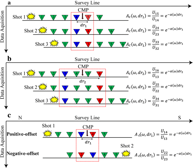

  

  Schematic diagram of method to extract amplitude ratio A _c in Eq. 3. a CMP with minimum receiver spacing dr ₁ and b CMP with larger receiver spacing dr ₂. c Definitions of positive- and negative-offset data. Triangles represent receiver positions. In generating amplitude ratio data, the data with the longer offset (red) are divided by the data with shorter offset (blue)

• 5. The value of α can be estimated by the linear regression of dr versus ln(A _c) (e.g., Foti et al. 2014) through the origin.

• 6. By performing steps 4 and 5 for other CMPs, local attenuation coefficients α can be obtained as a function of the CMPs.

In their two-dimensional attenuation analysis, Bergamo and Socco (2014) separately estimated local attenuation coefficients for each shot because the seismic energy at a reference point, corresponding to the intercept of their linear regression for estimating attenuation coefficients, differs from each shot. In our proposed method, however, we can simultaneously use multishot data in estimating local attenuation coefficients because the initial source amplitude is canceled out in generating the amplitude ratio gather with Eq. 3, and the amplitude ratio gather does not depend on the source amplitude or source location. Also, the midpoints between receiver pairs in the amplitude ratio data are coincident with local points (CMPs). Therefore, local points can be assigned greater weight, compared with the previous attenuation analysis.

In the presence of sharp discontinuities (e.g., faults), scattered surface waves can be observed (e.g., Xia et al. 2007; Hyslop and Stewart 2013; Strobbia et al. 2014; Bergamo and Socco 2014; Hyslop and Stewart 2015). In such laterally heterogeneous media, estimated values of α not only reflect attenuation coefficients related to quality factors but also include the effect of scattering (e.g., reflection) due to lateral heterogeneity. To detect lateral discontinuities, Bergamo and Socco (2014) utilized lateral variation of attenuation coefficients related to scattered surface waves. They estimated two attenuation coefficients at each local point (i.e., CMP in this study) from positive- and negative-offset data (e.g., Fig. 1c). Their results demonstrated that a distinct difference between the lateral variation of attenuation coefficients from positive- and negative-offset data is a good indication of the locations of a sharp lateral discontinuity. To effectively characterize lateral heterogeneities, we also focus on spatial variation of local attenuation coefficients related to scattering and separately estimate attenuation coefficients at each CMP from positive- and negative-offset data.

Numerical experiments

To characterize subsurface heterogeneities by the proposed attenuation method, we conducted numerical experiments for a model with a lithological boundary and a model with a fracture zone (Fig. 2). We investigated the difference between the local phase velocity and the attenuation coefficient in their sensitivity to these heterogeneities. The fracture zone is simulated as a low-velocity zone 6 m wide (Fig. 2d). P–SV waves are computed by a velocity-stress staggered grid using the finite-difference method with fourth-order spatial operators and a second-order temporal operator (Moczo 1998; Levander 1988). We apply a free-surface condition (Levander 1988) for the upper boundary and an absorbing boundary condition (Cerjan et al. 1985) for other boundaries. To focus on the spatial variation of local attenuation coefficients associated with structural heterogeneities, we neglect the effect of anelastic attenuation. In the simulation, seismic waves are recorded with 4-m receiver spacing and 2-m source spacing. The sources and receivers are located at the surface grids. Considering the offset range used in field data analysis, we analyze seismic data within the offset range from 16 to 200 m. The 10 Hz Ricker wavelet is used for a source function and added to the normal component of stress parallel to vertical direction. Other parameters are summarized in Table 1. Note that the actual simulation models are larger than the models shown in Fig. 2 to avoid artificial reflections from the boundaries (see Table 1).

Fig. 2

Diagrams showing the simulated models with examples of shot gathers. a–c Lithological boundary model. d–f Fracture model. V _p, V _s, and ρ are P-wave velocity, S-wave velocity, and density, respectively. Stars represent source positions. The origin time is defined at the maximum amplitude of the source wavelet

Table 1 Parameters of P-SV finite-difference modeling for the simulated models

We define CMP positions at every 10 m. We also define positive- and negative-offset data for the sources at the left and right sides of the CMPs, respectively (Fig. 1c). CMPCC gathers and amplitude ratio gathers are computed at each CMP. Phase velocities at each CMP are obtained by applying the MASW for the CMPCC gathers, in which the number of receiver pairs is given as the weighting function to enhance lateral resolution (Ikeda et al. 2013). At each CMP, attenuation coefficients are obtained from the linear regression of the amplitude ratio data, in which we use mean values of the observed amplitude ratio data within 8-m receiver spacing bins in a natural logarithmic scale. Bins with fewer than 10 data samples are discarded. Note that we did not apply the correction of geometrical spreading in Eq. (2) because of the absence of geometrical spreading of surface waves in 2D modeling.

In the model with a lithological boundary (Fig. 2a), we observed energy reflection at the boundary when the source was on the left side (i.e., low S-wave velocity zone) (Fig. 2b). When the source was on the right side (i.e., high S-wave velocity zone), we also observed energy reflection, but the reflection was small (Fig. 2c). Surface waves propagating from right to left (rigid–soft material) were amplified at the boundary. Phase velocities estimated by the CMPCC analysis showed clear lateral variation associated with the difference in lithology (Fig. 3a–c). The estimated phase velocities were weakly dependent on source directions. On the other hand, the lateral variation of estimated attenuation coefficients showed a clear dependence on the source direction (Fig. 3d–f). With positive-offset data, the estimated attenuation coefficients increased around the lithological boundary (Fig. 3e) as a result of energy reflection at the boundary. With negative-offset data, the attenuation coefficients decreased (Fig. 3f) by amplification at the boundary.

Fig. 3

Estimated phase velocities and attenuation coefficients for the lithological boundary model. a–c Phase velocities at each horizontal distance estimated from both-, positive- and negative-offset data, respectively. d–f Attenuation coefficients at each horizontal distance estimated from both-, positive- and negative-offset data, respectively

In the model with a fracture zone (Fig. 2d), we observed energy reflection at the fracture zone (Fig. 2e, f). Although the estimated phase velocities fluctuated slightly due to the existence of the fracture zone (Fig. 4a–c), locating the fracture zone was not straightforward. The attenuation coefficients increased near the fracture zone (Fig. 4d–f). The fracture zone could be characterized as a set of locations with low lateral variation in phase velocities and an increasing trend in attenuation coefficients.

Fig. 4

Estimated phase velocities and attenuation coefficients for the fracture model. a–c Phase velocities at each horizontal distance estimated from both-, positive- and negative-offset data, respectively. d–f Attenuation coefficients at each horizontal distance estimated from both-, positive- and negative-offset data, respectively

Thus, our numerical experiments clearly demonstrated differences between phase velocities and attenuation coefficients in their sensitivity to heterogeneities (whether lithological boundaries or fractures). Because the proposed attenuation analysis is based on the theory of one-way surface wave propagation, backscattered surface waves are not included in the theory. However, our results showed that the lateral heterogeneity associated with backscattered surface waves can be characterized as the lateral variation of attenuation coefficients. We use such apparent attenuation coefficients to detect heterogeneities in the following field data analysis.

Application to field data

To characterize subsurface heterogeneities from field data, we applied our proposed method to a dataset acquired near the MTL in western Shikoku Island, Japan (Fig. 5). This area contains two types of faults (e.g., Ikeda et al. 2009; Fig. 5b–d). One is the Kawakami fault, part of the MTL active fault system (MTLAFS). The other is the lithological boundary fault between Ryoke metamorphic rocks and Sambagawa metamorphic rocks (the material boundary MTL: MBMTL). Multichannel seismic data were acquired along a 1-km survey line with ~4-m receiver spacing and ~2-m source spacing as part of a reflection survey in an investigation of fault geometry on the MTL (Shigei et al. 2014). An impactor was used as a seismic source, and 30 Hz geophones were used as a receiver. Ikeda et al. (2013) estimated the two-dimensional S-wave velocity structure from the same dataset by the CMPCC analysis of surface waves (Fig. 5d). An example of the CMPCC gather and frequency-wavenumber (phase velocity) spectrum estimated by Ikeda et al. (2013) is shown in Additional file 1: Figure S1.

Fig. 5

Location map of Japan showing seismic profile and its S-wave velocity structure. a Location of Shikoku Island. b Geology and tectonic features of Shikoku [modified from Ikeda et al. (2009)]. c Detail of b showing the survey line (gray), the portion of the survey line used in this study (black), MTLAFS (red), and MBMTL (blue). d S-wave velocity structure of the seismic profile segment used in this study [modified from Ikeda et al. (2013)]

We analyzed a length of ~400 m along the survey line around the MBMTL and MTLAFS (Fig. 5c) and seismic data within the offset range from 15 to 200 m. CMPs were defined every 10 m using 2-m bins along the survey line. Positive- and negative-offset data were defined for sources to the north and south of the CMPs, respectively (Fig. 1c). To separate positive- and negative-offset data, we analyzed amplitude ratio data if the angle between the source-CMP direction and the direction of the receiver pairs for the amplitude ratio calculation was <30°. Additional file 2: Figure S2 plots the number of receiver pairs included in each CMP. At the north end of the profile, the number of receiver pairs for negative-offset data was small because of the survey (source-receiver) geometry (Additional file 2: Figure S2). Therefore, we show the results of negative-offset data analysis only for CMPs located more than 150 m from the north end of the survey line (Fig. 5c). We calculated mean values of the observed amplitude ratio data within 8-m bins in a natural logarithmic scale (see details in Fig. 6), discarding bins with fewer than 10 data samples.

Fig. 6

Observed amplitude ratio gathers at 15.1 Hz (natural logarithmic scale). The CMP is located at 220-m horizontal distance from the north end of the survey line (magenta square in Fig. 5c). a The observed amplitude ratio data with fit lines. Mean values and standard deviations (barred circles) are calculated from data (small crosses) within 8-m bins every 4 m. R ² values are calculated by regression analysis through the origin (Eisenhauer 2003). b The horizontal locations of the CMP (red cross) and receivers (black circles) used for computing the mean value at 60-m receiver spacing (green in a). We used receiver pairs from 56- to 64-m receiver spacing range (8-m bins) with the CMP at 220 m

At the CMP at 220 m on the profile (magenta square in Fig. 5c), the mean values of observed amplitude ratio data at 15.1 Hz from positive- and negative-offset data were well consistent with the corresponding fit lines (Fig. 6a). The negative value of attenuation coefficient α estimated from negative-offset data could not be explained by frequency-dependent attenuation of surface waves propagating in laterally homogeneous media, but they could appear near lateral discontinuities as a result of amplification at the boundary (Fig. 3f). The estimated attenuation coefficient from positive-offset data showed the opposite trend (positive value) consistent with the effect of scattering associated with a sharp lateral discontinuity (Bergamo and Socco 2014; Fig. 3e).

To investigate the vertical variation of α, estimated values of α were plotted as a function of one-third wavelength (roughly corresponding to depth) at each CMP (Fig. 7a, b; Additional file 3: Figure S3a, b) because depth sensitivity of Rayleigh waves is concentrated at about one-third wavelength (e.g., Hayashi 2008). In the conversion from frequency to depth, we also considered the effect of topography. The wavelengths for each CMP were obtained from the fundamental mode of dispersion curves estimated by the CMPCC analysis by Ikeda et al. (2013) (Fig. 7d; Additional file 1: Figure S1b; Additional file 3: Figure S3c). Note that the CMPCC analysis by Ikeda et al. (2013) used positive- and negative-offset data simultaneously in the phase velocity estimation for each CMP.

Fig. 7

Profiles of attenuation coefficients, their derivative values, and phase velocities. Profile location is shown in Fig. 5c. Values of α at 10-m intervals are estimated from amplitude ratio gathers for a positive-offset data and b negative-offset data. c Derivative values of the averaged values of α from 40- to 50-m elevation. d Fundamental mode of phase velocities (Ikeda et al. 2013). Depths are estimated as one-third of the wavelengths of phase velocities obtained by Ikeda et al. (2013). Black lines represent the ground surface. Background color shading is obtained from observed values (dots) by linear interpolation. The figure without the color shading is displayed in Additional file 3: Figure S3

At ~250 m on the profile in Fig. 7, we observed an abrupt change in the values of α estimated from positive- and negative-offset data (Fig. 7a, b). Values of α from positive-offset data decreased with distance along the profile, opposite to their trend from negative-offset data. To evaluate the degree of change in α with horizontal direction, we examined the derivative values of α with respect to horizontal distance (Fig. 7c), calculated from the average value of α over 40- to 50-m elevation. The derivative values of α calculated from positive- and negative-offset directions had large values but opposite signs at ~250 m. This contrast in opposite attenuation trends marks the locations of sharp lateral discontinuities (Bergamo and Socco 2014) caused by scattering or amplification at the boundary (Fig. 3e, f) and, indeed, the lithological boundary on the MTL (MBMTL) near here (Figs. 5c, 7). Lateral variation near the MBMTL is apparent in the dispersion curves of Fig. 7d.

At ~150-m horizontal distance, we also observed an abrupt change in the values of α estimated from positive-offset data (Fig. 7a), although we had no negative-offset data here (Fig. 7b; Additional file 2: Figure S2). The increasing trend also corresponded to large derivative values (Fig. 7c). A plausible cause of this lateral variation of α is the nearby Kawakami fault (MTLAFS; Figs. 5c, 7). Interestingly, phase velocity data could not resolve this discontinuity because the dispersion curves near the MTLAFS do not show clear lateral variations (Fig. 7d). Our result agrees with the simulation study for the fracture model (Fig. 4).

We also observed vertical, frequency-dependent variation of the estimated attenuation coefficients mainly caused by S-wave quality factors (e.g., Xia et al. 2002). The values of α generally decrease with increasing wavelength (pseudo-depth) as clearly seen on the south side of the negative-offset result (Fig. 7b).

As with phase velocity estimation, there is a trade-off between spatial resolution and the length of a moving window when estimating attenuation coefficients at a local point (Bergamo and Socco 2014). Longer receiver spacing yields more reliable attenuation coefficients, whereas the effect of lateral heterogeneity around a CMP can be reduced by excluding data with longer receiver spacings. As Ikeda et al. (2013) demonstrated in CMPCC analysis, the spatial window can be applied for our proposed attenuation method. In this study, the maximum receiver spacings were about 180 m at each CMP. In our field example, lateral variation in the estimated values of α north of 300 m on the profile was similar when the maximum receiver spacings were reduced to 100 m (Additional file 4: Figure S4), but the opposite trend in the estimated values of α appeared south of 300 m. This opposite trend might be related to lateral discontinuities other than MBMTL and MTLAFS.

Discussion

When we applied our proposed method to field data, we estimated significant lateral variations in attenuation coefficient α at locations matching two faults, MBMTL and MTLAFS, in the study area (Fig. 7a–c). However, a study using phase velocities (Ikeda et al. 2013) showed significant lateral variation only at the fault that constitutes a lithological boundary (MBMTL, Fig. 7d). The lateral variation in phase velocities estimated by surface wave analysis mainly reflects lithological differences (most sensitive to differences in S-wave velocities) (e.g., Fig. 3a–c and MBMTL; Fig. 7d). Because the effects of backscattered surface waves with negative-phase velocities can be reduced in frequency-wavenumber analysis (e.g., MASW), the effect of scattering due to lateral discontinuities (lithological boundaries or localized fractures) is suppressed in phase velocity estimations. Furthermore, since the resolution of phase velocity estimation is not enough to resolve the localized fracture (i.e., small-scale velocity anomaly), clear lateral variation cannot be observed in the estimated phase velocities around localized fractures (Fig. 4a–c and MTLAFS; Fig. 7d). On the other hand, attenuation coefficients vary as a result of both lithological differences and localized fractures (Figs. 3d–f, 4d–f, 7a, b). Around the MTLAFS, scattering by the fracture would be dominant in the estimated attenuation coefficients because the phase velocity result would not detect a lithological contrast. The estimated attenuation coefficients increased near the MTLAFS (Fig. 7a) as the simulation study also showed (Fig. 4d–f), whereas the effect of scattering and amplification at the lithological boundary was indicated near the MBMTL from the opposing trends in the α estimated from positive- and negative-offset data (Figs. 3e, f, 7a–c).

However, we observed a single high-attenuation anomaly between the MTLAFS and MBMTL (Fig. 7a). Because of the absence of the negative-offset result around the MTLAFS, the contribution of the fracture (i.e., MTLAFS) for the attenuation anomaly is not clear. To investigate the contribution of the fracture, we performed a simulation of the inverted velocity model based on phase velocity analysis (Ikeda et al. 2013; Fig. 5d) by the same procedure in the section of numerical experiments.

The simulated model did not include a fracture zone, thus allowing the effects of its absence to be tested. However, the difference between the simulation and the field test was also influenced by anelastic attenuation, which was included only in the field experiment. To reduce the effect of such frequency-dependent attenuation, we compute the normalized average attenuation coefficients $\alpha_{{lm, {\text{norm}}}}$ for frequency f _m and the lth CMP based on Bergamo and Socco (2014),

$$\alpha_{{lm, {\text{norm}}}} = \frac{{\alpha_{lm} -\left\langle\alpha_{m}\right\rangle}}{{{\text{stdev}}(\alpha_{m} )}},$$

(4)

where α _lm is the attenuation coefficient for f _m and the lth CMP, $\left\langle {\alpha _{m} } \right\rangle$ is the mean value of the attenuation coefficients among all CMPs for f _m , and stdev(α _m ) is the standard deviation of that mean value. The normalized attenuation coefficients can emphasize the lateral variation of attenuation coefficients and reduce the effect of frequency-dependent attenuation coefficients.

We compared the normalized attenuation coefficients obtained from the simulation with those from the field data analysis in Fig. 8. Near the MBMTL, both analyses showed opposing trends in positive- and negative-offset data and a single high-attenuation anomaly in positive-offset data. At high frequencies, the high-attenuation anomaly in the simulation result in positive-offset data (Fig. 8a) was shifted to the south, compared with the field result (Fig. 8c). They also differ in that a dipping high-attenuation structure appeared in the simulation result for positive-offset data near the MBMTL (arrow in Fig. 8a), and this structure appeared to be related to the slope of the lithological boundary identified in S-wave velocity data (Figs. 5d, 7d). However, this structure was absent in field data analysis (Fig. 8c).

Fig. 8

Comparison of normalized attenuation coefficients estimated from the numerical simulation (a, b) with those from field data (c, d). Black dots represent points where the fundamental mode of surface waves can be estimated in phase velocity analysis by Ikeda et al. (2013)

Since the MBMTL and MTLAFS obliquely cross the survey line (Fig. 5c), reflected surface waves from lateral direction for the survey line would influence the lateral variation of the estimated attenuation coefficients. To investigate such 3D effects, we further performed 3D numerical simulation using the staggered-grid finite-difference method with fourth-order spatial operators and a second-order temporal operator as shown in Graves (1996). Following the description in Moczo (1998), we extended the 2D numerical simulator used in the section of numerical experiments for 3D media. The 3D model was constructed by extending the 2D velocity model in Fig. 5d along the MTLs. Because of the limited computational capacity, we reduced the number of the grid cell and increased the grid size from 1 to 2 m. In this condition, synthesized waveforms would be stable up to 28 Hz, assuming that at least five grid spacings are used to sample the wavelength (Moczo 1998). We also changed the shot interval from 2 to 8 m and computed synthesized shot gathers with 4-m receiver spacing along the survey line. Other parameters used for 3D numerical simulation are summarized in Table 2.

Table 2 Parameters of 3D finite-difference modeling for the simulated model

As we expected, reflected surface waves from horizontal direction were observed in the synthesized waveforms (Fig. 9; Additional file 5: Video S1 for sequential snapshots). We estimated the lateral variation of normalized attenuation coefficients along the survey line (Fig. 10a, b). To compare the estimated attenuation coefficients from 3D simulation with those from 2D simulation, we estimated normalized attenuation coefficients for 2D simulation with 8-m shot interval (Fig. 10c, d). In the 3D simulation result for positive-offset data (Fig. 10a), we could observe the dipping structure of the high-attenuation anomaly although it was smeared and shifted to the north (dashed arrow in Fig. 10a). The attenuation anomaly at high frequencies was also slightly shifted to the north. However, it was still located near the MBMTL. Thus, our 3D simulation study indicated that reflected surface waves from lateral direction induced the shift of the high-attenuation anomaly including the dipping structure to the north, but the shift was not enough to explain the difference between the simulation and field results.

Fig. 9

Example of snapshots of vertical particle velocity field. a Horizontal slice at the surface and b, c two vertical slices at 1.195 s from the origin time defined at the maximum amplitude of the source wavelet. The vertical slices are defined along the dashed lines in a. The survey line is defined along the dashed line at y distance from 0 to 420 m. Red–blue color indicates the vertical particle velocity field. Stars represent source positions. We provide the sequential snapshots as the Additional file 5: Video S1

Fig. 10

Comparison of normalized attenuation coefficients estimated from the 3D numerical simulation (a, b) and 2D numerical simulation (c, d). The shot intervals used for both simulation results are 8 m. The solid arrows in a, c are located at the same positions as in Fig. 8a

Compared with the results of 2D or 3D numerical simulation, the dipping attenuation structure was masked and the high-attenuation anomaly was shifted to the north in the field results of positive-offset data. Because the fault is branched into several planes in the shallow formation due to low effective pressure (Tsuji et al. 2014), the fracture zone could be developed along the trace of large fault (i.e., MTL). Therefore, the fracture zone associated with the MTL fault system has possibility to cause increase in attenuation coefficients in the field data case (Fig. 8c). If so, it would increase the attenuation coefficients between the MTLAFS and MBMTL and mask the dipping attenuation structure observed in the simulation results for positive-offset data (Figs. 8a, 10a, c). Because of well-developed fracture zone, the high-attenuation zone in the simulation results would be shifted to the north, where it would coincide with the result of the field data analysis (Fig. 8c).

The presence of a fracture zone near the MTLAFS enables us to explain the differences between the attenuation coefficients from the simulation and the field data analysis. Thus, both a fracture and a lithological boundary are possibly needed to account for the lateral variation of the estimated attenuation coefficients in the field data.

However, we also observed the difference between the simulation and field results for negative-offset data (Figs. 8b, d, 10b, d). In the simulation results, we observed a dipping low-attenuation anomaly near the MBMTL, probably related to the slope of the lithological boundary. It is difficult to clearly explain the reason for the absence of the dipping structure in the field results of negative-offset data. Since the effect of surface wave attenuation is not considered in constructing the simulated model (Fig. 5d), the difference could be caused by sensitivity differences between the attenuation and phase velocity to localized structural heterogeneities. Although we computed normalized attenuation coefficients to reduce the effect of frequency-dependent attenuation coefficients, such anelastic attenuation included in only field data would also be responsible for the difference.

Because attenuation coefficients has the possibility to resolve localized fractures (Fig. 8c), our proposed method provides crucial information in fluid injection experiments (e.g., CO₂ storage), in which localized fractures that may leak fluids are undesirable. Our proposed method creates the potential to detect such localized fractures using conventional surface seismic data.

Summary

To characterize subsurface heterogeneities, we proposed a method for estimating spatial variation in attenuation coefficients of surface waves from multichannel–multishot data. Like the CMPCC analysis proposed by Hayashi and Suzuki (2004), this method retains high lateral resolution while estimating attenuation coefficients at each CMP. In this method, multishot data can be easily combined because source amplitude of each shot is canceled out in estimating the local attenuation coefficients.

Our study demonstrated that the lateral variation of attenuation coefficients estimated by the proposed method can identify sharp lateral discontinuities such as lithological boundaries and fracture zones. Estimating attenuation coefficients separately from positive- and negative-offset data is effective in identifying lithological boundaries. We also demonstrated that attenuation coefficients are more sensitive to localized fractures than phase velocities, although both attenuation coefficients and phase velocities are sensitive to lithological boundaries. Therefore, simultaneous interpretation of lateral variation of attenuation coefficients and that of phase velocities has a potential to distinguish lithological boundaries from the localized lateral discontinuities (fractures associated with faults). This ability would be valuable in applications such as fluid injection studies, where it may allow localized fractures to be detected using conventional seismic data.

References

Bergamo P, Socco LV (2014) Detection of sharp lateral discontinuities through the analysis of surface-wave propagation. Geophysics 79(4):EN77–EN90
Bergamo P, Boiero D, Socco LV (2012) Retrieving 2D structures from surface-wave data by means of space-varying spatial windowing. Geophysics 77(4):EN39–EN51
Boiero D, Socco LV (2010) Retrieving lateral variations from surface wave dispersion curves. Geophys Prospect 58(6):977–996
Cerjan C, Kosloff D, Kosloff R, Reshef M (1985) A nonreflecting boundary condition for discrete acoustic and elastic wave equations. Geophysics 50:705–708
Eisenhauer JG (2003) Regression through the origin. Teach Stat 25(3):76–80
Foti S (2004) Using transfer function for estimating dissipative properties of soils from surface-wave data. Near Surf Geophys 2(4):231–240
Foti S, Lai CG, Rix GJ, Strobbia C (2014) Surface wave methods for near-surface site characterization. CRC Press, Boca Raton
Graves RW (1996) Simulating seismic wave propagation in 3D elastic media using staggered-grid finite differences. Bull Seismol Soc Am 86(4):1091–1106
Hayashi K (2008) Development of surface-wave methods and its application to site investigations. Ph.D. dissertation, Kyoto University
Hayashi K, Suzuki H (2004) CMP cross-correlation analysis of multi-channel surface-wave data. Explor Geophys 35(1):7–13
Hyslop C, Stewart R (2013) Imaging faults using reflected surface waves. In: SEG technical program expanded abstracts 2013, Huston, TX, USA, 22–27, September, pp 1728–1732
Hyslop C, Stewart R (2015) Imaging lateral heterogeneity using reflected surface waves. Geophysics 80(3):EN69–EN82
Ikeda M, Toda S, Kobayashi S, Ohno Y, Nishizaka N, Ohno I (2009) Tectonic model and fault segmentation of the Median Tectonic Line active fault system on Shikoku, Japan. Tectonics 28:TC5006. doi:10.1029/2008TC002349
Ikeda T, Tsuji T, Matsuoka T (2013) Window-controlled CMP crosscorrelation analysis for surface waves in laterally heterogeneous media. Geophysics 78(6):EN95–EN105
Lai CG, Rix GJ, Foti S, Roma V (2002) Simultaneous measurement and inversion of surface wave dispersion and attenuation curves. Soil Dyn Earthq Eng 22(9):923–930
Levander AR (1988) Fourth-order finite-difference P–SV seismograms. Geophysics 53:1425–1436
Lin F-C, Ritzwoller MH, Shen W (2011) On the reliability of attenuation measurements from ambient noise crosscorrelations. Geophys Res Lett 38:L11303
Misbah AS, Strobbia CL (2014) Joint estimation of modal attenuation and velocity from multichannel surface wave data. Geophysics 79(3):EN25–EN38
Moczo P (1998) Introduction to modeling seismic wave propagation by the finite-difference method. Lecture Notes. Disaster Prevention Research Institute, Kyoto University
Nasseri-Moghaddam A, Cascante G, Hutchinson J (2005) A new quantitative procedure to determine the location and embedment depth of a void using surface waves. J Environ Eng Geophys 10(1):51–64
Park CB, Miller RD, Xia J (1998) Imaging dispersion curves of surface waves on multi-channel record. In: SEG technical program expanded abstracts 1998, New Orleans, LA, USA, 14–18, September, pp 1377–1380
Park CB, Miller RD, Xia J (1999) Multichannel analysis of surface waves. Geophysics 64(3):800–808
Saito H, Hayashi K, Iikura Y (2004) Detection of formation boundaries and permeable fractures based on frequency-domain Stoneley wave logs. Explor Geophys 35:45–50
Shigei Y, Tsuji T, Matsuoka T, Ikeda M, Nishizaka N, Ishikawa Y (2014) Seismic-derived quality factor for lithology classification around the median tectonic line. J Soc Mater Sci Jpn 63(3):250–257 (in Japanese with English abstract)
Socco LV, Foti S, Boiero D (2010) Surface-wave analysis for building near-surface velocity models—established approaches and new perspectives. Geophysics 75(5):75A83–75A102
Strobbia C, Foti S (2006) Multi-offset phase analysis of surface wave data (MOPA). J Appl Geophys 59(4):300–313
Strobbia C, Zarkhidze A, May R, Ibrahim F (2014) Model-based attenuation for scattered dispersive waves. Geophys Prospect 62(5):1143–1161
Tsuji T, Johansen TA, Ruud BO, Ikeda T, Matsuoka T (2012) Surface-wave analysis for identifying unfrozen zones in subglacial sediments. Geophysics 77(3):EN17–EN27
Tsuji T, Kamei R, Pratt G (2014) Pore pressure distribution of a mega-splay fault system in the Nankai Trough subduction zone: insight into up-dip extent of the seism genic zone. Earth Planet Sci Lett 396:165–178
Werning M, Boiero D, Vermeer P (2013) Q estimation for surface waves. In: 75th EAGE conference and exhibition incorporating SPE EUROPEC 2013, London, UK, 10–13, June, Th-01-02
Xia J, Miller RD, Park CB (1999) Estimation of near-surface shear-wave velocity by inversion of Rayleigh waves. Geophysics 64(3):691–700
Xia J, Miller RD, Park CB, Tian G (2002) Determining Q of near-surface materials from Rayleigh waves. J Appl Geophys 51(2):121–129
Xia J, Nyquist JE, Xu Y, Roth MJ, Miller RD (2007) Feasibility of detecting near-surface feature with Rayleigh-wave diffraction. J Appl Geophys 62(3):244–253
Xia J, Miller RD, Ivanov J, Zeng C (2009) High-frequency Rayleigh-wave method. J Earth Sci 20(3):563–579
Zerwer A, Polak MA, Santamarina JC (2005) Detection of surface breaking cracks in concrete members using Rayleigh waves. J Environ Eng Geophys 10(3):295–306
Authors’ contributions
TI carried out the data analysis and drafted the manuscript. TT joined the methodological discussion and helped to draft the manuscript. Both authors read and approved the final manuscript.
Acknowledgements
We thank Editor Hiroshi Takenaka and two anonymous reviewers for constructive comments that improved manuscript. We also thank Shikoku Electric Power Co., Inc., and Shikoku Research Institute Inc., for seismic data acquired across the MTL. This study was done in collaboration with Shikoku Research Institute Inc. We gratefully acknowledge the support provided by the International Institute for Carbon Neutral Energy Research, sponsored by the World Premier International Research Center Initiative, MEXT, Japan.
Authors’ information
TI received a B.S. (2009) in Global Engineering, M.Sc. (2011) in Civil and Earth Resources Engineering, and a Ph.D. (2014) in Urban Management from Kyoto University, Japan. Since 2014, he has been a postdoctoral research associate at the CO2 Storage Division of the International Institute for Carbon-Neutral Energy Research (WPI-I2CNER), Kyushu University. His research interests include surface wave analysis considering the effects of higher modes, lateral variation, attenuation, and anisotropy. TT received a B.S. (2002) in Resources Engineering from Waseda University, Japan, and an M.Sc. (2004) and a Ph.D. (2007) in Earth Science from the University of Tokyo, Japan. From 2007 to 2012, he was an assistant professor of Engineering Geology Group at Kyoto University. From 2010 to 2011, he stayed at Rock Physics Department of Stanford University. Since 2012, he has been an associate professor at Kyushu University. He is lead principal investigator at the CO2 Storage Division of the International Institute for Carbon-Neutral Energy Research (WPI-I2CNER). His research interests include seismic reflection and refraction analysis, surface wave analysis, seismic attributes analysis, rock physics, seismic anisotropy, seismic interferometry, and interferometric SAR.
Competing interests
Both authors declare that they have no competing interests.
Author information
Authors and Affiliations
Corresponding author
Additional files
40623_2016_487_MOESM1_ESM.png
Additional file 1: Figure S1. Example of the CMPCC gather and frequency-wavenumber spectrum estimated by Ikeda et al. (2013). The CMP is located at 90 m horizontal distance from the north end of the survey line. (a) The 20 Hz low-pass-filtered CMPCC gather. (b) Frequency-wavenumber (phase velocity) spectrum estimated from the CMPCC gather. Red circles represent estimated fundamental mode phase velocities.
40623_2016_487_MOESM2_ESM.png
Additional file 2: Figure S2. Numbers of receiver pairs in the amplitude ratio gathers for each horizontal distance (CMP). Profile location is shown on Figure 5c.
40623_2016_487_MOESM3_ESM.png
Additional file 3: Figure S3. Profiles of attenuation coefficients and phase velocities. Same as Figures 7a, b, and d but without background shading.
40623_2016_487_MOESM4_ESM.png
Additional file 4: Figure S4. Profiles of attenuation coefficients and their derivative values. Same as Figures 7a-c but using the amplitude ratio data with receiver spacing less than 100 m.
40623_2016_487_MOESM5_ESM.mp4
Additional file 5: Video S1. Movie of snapshots of 3D synthesized waveforms. This movie corresponds to shapshots in Figure 9. t in the movie indicates the time from the origin time defined at the maximum amplitude of the source wavelet. See the caption of Figure 9 for details.
Rights and permissions
Open Access This article is distributed under the terms of the Creative Commons Attribution 4.0 International License (http://creativecommons.org/licenses/by/4.0/), which permits unrestricted use, distribution, and reproduction in any medium, provided you give appropriate credit to the original author(s) and the source, provide a link to the Creative Commons license, and indicate if changes were made.
About this article
Cite this article
Ikeda, T., Tsuji, T. Surface wave attenuation in the shallow subsurface from multichannel–multishot seismic data: a new approach for detecting fractures and lithological discontinuities. Earth Planet Sp 68, 111 (2016). https://doi.org/10.1186/s40623-016-0487-0
Received:
Accepted:
Published:
DOI: https://doi.org/10.1186/s40623-016-0487-0