A high-resolution gravimetric quasigeoid model for Vietnam

Abstract

A high-resolution gravimetric quasigeoid model for Vietnam and its surrounding areas was determined based on new gravity data. A set of 29,121 land gravity measurements was used in combination with fill-in data where no gravity data existed. Global Gravity field Models plus Residual Terrain Model effects and gravity field derived from altimetry satellites were used to provide the fill-in information over land and marine areas. A mixed model up to degree/order 719 was used for the removal of the long and medium wavelengths and the calculation of the quasigeoid restore effects. The residual height anomalies have been determined employing the Stokes integral using the Fast Fourier Transform approach and deterministic kernel modification proposed by Wong–Gore, as well as by means of Least-Squares Collocation. The accuracy of the resulting quasigeoid models was evaluated by comparing with height anomalies derived from 812 co-located GNSS/levelling points. Results are very similar; both local quasigeoid models have a standard deviation of 9.7 cm and 50 cm in mean bias when compared to the GNSS/levelling points. This new local quasigeoid model for Vietnam represents a significant improvement over the global models EIGEN-6C4 and EGM2008, which have standard deviations of 19.2 and 29.1 cm, respectively, for this region.

Introduction

The quasigeoid is defined as a surface that is the closest to mean sea level (Hofmann-Wellenhof and Moritz 2006). It serves as a reference surface for the vertical system (Torge and Müller 2012). The normal height (H^*), the geometric distance between the quasigeoid and the Earth’s surface, has traditionally been determined by spirit levelling and adding the normal correction in order to transform the levelled height into the normal height, but it has taken much time and cost. Thanks to GNSS technology, accurate ellipsoidal heights (h) are now easily accessible and the normal height can also be determined by subtracting the height anomaly (ζ) from the geodetic height as follows:

$$H^{*} = h - \zeta$$

(1)

For local or regional applications, the efficiency of this approach is valid only if the height anomalies are known with an accuracy of few centimetres. In Vietnam, Global Gravity field Models (GGM) have been used in GNSS applications since the late 1990s: EGM96 (Lemoine et al. 1998) at first and currently EGM2008 (Pavlis et al. 2012). However, EGM2008 is inadequate for GNSS levelling over Vietnam. Its accuracy is insufficient to comply with fourth-order levelling specifications (a misclosure of $25\sqrt {\mathrm{k}}$ mm over a distance of k km). A local gravimetric quasigeoid of Vietnam was so far never calculated. So, there is a strong need for a high-accuracy and high-resolution gravimetric quasigeoid model of Vietnam and its vicinity for the purpose of modernizing the height system using GNSS instead of spirit levelling, as well as for other applications such as geology, geophysics, and oceanography. Several neighbouring countries make continuous efforts to determine and improve their geoid or quasigeoid model successfully. For comparison, Table 1 shows the accuracy of several local geoid or quasigeoid models, and notably of neighbouring countries in Asia. The resulting standard deviations (STD) obtained for the most recent geoids models range from a few cm up to 30 cm, depending on the quality of the available gravity data for the quasigeoid determination. Note that a hybrid model is constructed using a gravimetric geoid or quasigeoid and GNSS/levelling data.

Table 1 Statistics of selected local geoid or quasigeoid models

Presently, all conditions for accurate high-resolution quasigeoid determination using the Remove–Compute–Restore (RCR) technique (Sansò and Sideris 2013) of Vietnam are met thanks to:

• A new generation of Global Gravity Field Models (GGM) based on Gravity field and steady-state Ocean Circulation Explorer (GOCE; Drinkwater et al. 2003) data was developed;

• High-resolution Digital Terrain Models (DTM);

• New gravity measurements covering the entire country, even if not homogeneously, as well as high-resolution altimeter-inferred gravity anomaly data over sea.

The objective of this study is to compute a gravimetric quasigeoid model of Vietnam with an accuracy that allows GNSS levelling to comply with fourth- or maybe third-order levelling specifications. High-quality GNSS/levelling data were used to assess the accuracy of the developed quasigeoid models.

This paper describes the development and validation of quasigeoid solutions for Vietnam. Because gravity data are not available for Vietnam’s neighbouring countries, this paper will only focus on modelling the quasigeoid of Vietnam. “Quasigeoid determination methodology” section briefly presents the two methods used to compute the quasigeoid, namely the Stokes’ integral—Fast Fourier Transform (FFT), and Least-Squares Collocation (LSC). “Data and pre-processing” section describes the data and the procedure for pre-processing the data. “Quasigeoid model estimation and validation” section presents and discusses results of the quasigeoid computations. Finally, “Conclusions” section gives the conclusions on the development and accuracy of the quasigeoid of Vietnam.

Quasigeoid determination methodology

The RCR technique is a well-known method for gravimetric quasigeoid determination. It is realized by summation of three terms according to the formula:

$$\zeta = \zeta_{\mathrm{GGM}} + \zeta_{\mathrm{RTM}} + \zeta_{\mathrm{res}}$$

(2)

where ζ_GGM is computed using a global geopotential model, ζ_RTM expresses the Residual Terrain Model (RTM) effect, and ζ_res is computed from residual gravity anomalies employing the Stokes’ integral or LSC. The residual gravity anomalies used to determine ζ_res are computed as follows:

$$\Delta g_{\mathrm{res}} = \Delta g_{\mathrm{FA}} - \Delta g_{\mathrm{GGM}} - \Delta g_{\mathrm{RTM}}$$

(3)

where $\Delta g_{\mathrm{FA}}$ is the free-air gravity anomaly, $\Delta g_{\mathrm{GGM}}$ is the gravity anomaly computed with a GGM, and $\Delta g_{\mathrm{RTM}}$ is the RTM effect on the gravity anomaly.

In this study, we used the GRAVSOFT software (Forsberg and Tscherning 2008) developed at DTU (Technical University of Denmark) to perform the quasigeoid computations. The gravity anomaly and height anomaly were computed using the GRAVSOFT GEOCOL program. The RTM effects on the gravity anomaly and the height anomaly were computed using the GRAVSOFT TC program, with a radius of 20 km for the detailed DTM and 200 km for the coarse grid. Thus, we need three models to calculate the RTM effects with TC program; these are the detailed (SRTM3arc), coarse, and reference DTMs in which the reference height grid was estimated by low-pass filtering the detailed DTM in order to represent the topographic signal above the maximum degree of the GGM used (Forsberg 1984). The coarse and reference DTM models were created as follows:

• The coarse grid is computed by simple averaging (e.g. 3′ × 3′ grid) of the detailed DTM model using the SELECT program.

• The coarse grid (3′ × 3′) is then filtered with a moving average operator to the required resolution using the TCGRID program; in the remove–restore procedure, the required resolution is 27.8 km (equivalent to spherical harmonic d/o 720).

All computations have been performed with the reference ellipsoid WGS84, of which the constants are: a = 6,378,137.00 m, f = 1/298.257223563, GM₀ = 3.986004418 × 1014 m³ s⁻², and in the Tide Free (TF) system. When a GGM is referred to the Zero Tide (ZT) system or the Mean Tide (MT) system, the C_2,0 coefficient is converted to the TF system using the formula reported in Rapp (1989). In Vietnam, where the height system refers to the MT system, the conversion from MT system to the TF system is done according to Ekman (1989).

Data and pre-processing

The quasigeoid model was developed according to the diagram shown in Fig. 1, which presents the different steps, inputs, and modules for RCR operations. The input data are presented in the following sections.

Fig. 1

Diagram of sequential steps (top to bottom) in the calculation of the quasigeoid

Global Geopotential Models (GGM)

Gravity data are reduced for the long and medium wavelengths, using GGMs, and the terrain effect, using DTMs, in order for the residual gravity anomalies to be smooth before gridding or prediction. The GGM has to best represent the gravity anomalies and height anomalies in the selected area. GGMs, enhanced with RTM effects, are also used to generate fill-in data where gravity measurements are not available. The GGMs are available on the International Center for Global Earth Models (ICGEM) Web site.

The high-resolution EGM2008 model, developed up to degree/order (d/o) 2190, has well-known errors, due to datum inconsistencies and variability of the measurement density and accuracy (Gilardoni et al. 2013), in the low–medium frequency band because it is a pre-GOCE model. Moreover, as it includes a large variety of surface measurements, uncertainties also arise from datum inconsistency in the compiled gravity database and from variability of the measurement density and accuracy. In Gilardoni et al. (2013), a GOCE model was successfully used to improve the geoid model accuracy by combining spherical harmonic coefficients of the EGM2008 model with a GOCE gravity model. Following previous studies that successfully used mixed GOCE and EGM2008 models for the removal of the long and medium wavelengths to compute geoids of Malaysia (Jamil et al. 2017), Nepal (Forsberg et al. 2014a), and the Philippines (Forsberg et al. 2014b), we constructed a similarly combined model to remove the long to medium wavelength components of the gravity field up to d/o 719. We used the fifth release of GOCE global potential model obtained from the direct approach, named EGM-DIR-R5 (Bruinsma et al. 2014). The combination was done in the following way:

• Degrees 2-260: EGM-DIR-R5.

• Degrees 270-2190: EGM2008.

• The coefficients of the mixed model from degrees 260 to 270 are computed by weighted mean of the two models with the weights being determined as the inverse of degree variances. These coefficients are computed as follows (Gilardoni et al. 2013):

  $$T_{mn} = \left[ {\frac{{T_{mn}^{E} }}{{\left( {\sigma_{{T_{mn} }}^{2} } \right)^{E} }} + \frac{{T_{mn}^{D} }}{{\left( {\sigma_{{T_{mn} }}^{2} } \right)^{D} }} } \right]\left[ {\frac{1}{{\left( {\sigma_{{T_{mn} }}^{2} } \right)^{E} }} + \frac{1}{{\left( {\sigma_{{T_{mn} }}^{2} } \right)^{D} }} } \right]^{ - 1}$$

  (4)

  where $T_{mn}^{E}$ and $\left( {\sigma_{{T_{mn} }}^{2} } \right)^{E}$ are the coefficients and degree variances, respectively, derived from EGM2008. $T_{mn}^{D}$ and $\left( {\sigma_{{T_{mn} }}^{2} } \right)^{D}$ are the coefficients and degree variances, respectively, derived from EGM-DIR-R5.

All recent GGMs, such as GOCO05s (Mayer-Guerr 2015), EGM-TIM-R5 (Brockmann et al. 2014), and EGM-SPW-R5 (Gatti et al. 2016), were tested in this study, in steps of 10 degrees, to find out the best GGM and its optimum maximum degree in combination with EGM2008. Figure 2 indicates the STD of the differences between the GOCE GGMs in combination with EGM2008 and the GNSS/levelling data. The EGM-DIR-R5 at d/o 260 plus EGM2008 is the best model with the smallest STD of 0.16 m. Moreover, the EIGEN-6C4 model (Förste et al. 2014), computed from the combination of LAser GEOdynamics Satellite (LAGEOS), Gravity Recovery And Climate Experiment (GRACE), GOCE, and a reconstruction of EGM2008 beyond d/o 235, was also tested. The combination model described above best reproduces the gravity data. In particular, the Experimental Gravity Field Model XGM2016 (Pail et al. 2018), computed with improved terrestrial data especially over continental areas such as South America, Africa, parts of Asia, and Antarctica, up to the same d/o 719, was also used to compute quasigeoid for this region, but the result was slightly worse than when using the mixed model.

Fig. 2

Standard deviation of the differences between the GOCE GGMs in combination with EGM2008 and the GNSS/levelling data

Digital Terrain Models (DTM)

The DTM provides information on the short wavelengths of the gravity field. RTM was selected to calculate the terrain effects; using the RTM the smoothing effect on gravity data can reach 50% if their elevations are accurate (Forsberg 1984). Over land areas, the 90 m resolution SRTM3arc_v4.1 (Farr et al. 2007) was used as the detailed DTM. The 15” resolution Digital Bathymetry Model (DBM) SRTM15arc_plus (Becker et al. 2009) was used over sea, and after re-gridding to 3’’ it was then merged with SRTM3arc_v4.1 using the full-resolution coastline in Generic Mapping Tools (GMT) (Wessel and Smith 1998). Several DTMs, such as Earth2012 (Hirt 2013) and DTM2006 (Pavlis et al. 2012), were also used for computing residual gravity anomalies on land, but the best model is SRTM3arc_v4.1 (the STD of residual gravity anomalies using this model is the smallest). To avoid the need to distinguish between different density values (mass density of water ρ_w = 1030 kg m⁻³ and mass density of rock ρ_r = 2670 kg m⁻³), we used the Rock-Equivalent Topography (RET) approach (Balmino et al. 1973, 2012).

Gravity measurements and fill-in data

For the purpose of determining the quasigeoid, we collected terrestrial gravity data obtained from the Institute of Geophysics (IGP)—Vietnam Academy of Science and Technology (VAST), the Vietnam Institute of Geodesy and Cartography (VIGAC), and the Bureau Gravimétrique International (BGI; Bonvalot 2016). The total number of gravity points is 31,102. A set of 19,267 land gravity points was collected from IGP, but these surveys have been done between 1961 and 1984 for the purpose of geological survey, exploration geophysics, and mineral prospecting when positioning was of poor quality, especially for heights, which were determined using barometers (green points in Fig. 3). As errors in the elevation will propagate into the computed gravity anomaly, gross error detection methods were first applied to clean up the IGP data (see below). Fortunately, most of the countries have been re-surveyed from 2003 to 2011, through the project “Measurement and Improvement of Vietnam National Gravity Data”, carried out in collaboration with the Moscow Institute of Geodesy, Cartography and Aerial Images, Moscow State University of Geodesy and Cartography (MIIGAiK), Russia. This new dataset comprises 10,940 points, including an absolute gravity network of 11 base reference stations with an accuracy of better than ± 5 μGal and their tie points, 29 first-order gravity stations with an accuracy of better than ± 15 μGal and their tie points, and 92 third-order gravity points and more than 10,000 detailed points measured from 2005 to 2009 (red points in Fig. 3). The base reference stations and first-order gravity network were determined from absolute measurements using GBL instrument (Final Report of VIGAC 2012). For the VIGAC gravity surveys, GNSS has been used to determine coordinate and height, so this is less prone to errors in positioning. The IGP data are less accurate than the VIGAC data. However, the combination of the IGP and VIGAC data enhances the coverage considerably, especially in the South of Vietnam. Finally, our land gravity data set was also complemented by a set of gravity data provided by BGI for Vietnam and surrounding areas (including 895 points in Vietnam, 229 points in Cambodia, and 351 points in Thailand).

Fig. 3

Distribution of land gravity data used in this study: red dots are the VIGAC points, absolute points are indicated by triangles, green dots are the IGP points, and blue dots are obtained from the BGI database

We have used two procedures to detect localized gross errors in the data. The first uses SRTM3arc data to verify the gravity observation elevations in the IGP data. The results are listed in Table 2. The differences at GNSS/levelling points show a STD of 6.86 m and an average bias of − 3.13 m, which are in line with results of Denker (2005) in Germany. The VIGAC data show a STD of 23.46 m and average bias of − 4.23 m, while SRTM3arc has a reported vertical accuracy of better than 16 m (Farr et al. 2007). This proves that SRTM provides very good height information in the computation of the RTM effect. The differences of the gravity observation elevations in the IGP data with SRTM3arc are 73.50 m in STD and − 14.95 m in mean bias. This indicates that the elevations in the IGP data, which were determined from barometric levelling, have gross errors. A horizontal error in gravity data will also result in a discrepancy between the gravity observation elevations in the IGP data and those derived from DTM, especially in areas of steep elevation changes; consequently, we cannot use elevation derived from the DTM and we need a different procedure to detect gross errors in IGP data.

Table 2 Statistics of the differences between the observation elevations and the SRTM3arc [Unit: (m)]

The second procedure involves comparisons with the EGM-DIR-R5 model. To reduce the effect of the omission error in the GGM, we have used EGM-DIR-R5 augmented with high-resolution RTM effects beyond its selected resolution (degree 260). The RTM effects were computed using the GRAVSOFT TC program. The reference height grid was estimated in order to represent the topographic signal above degree 260 of EGM-DIR-R5. The 3” resolution of DTM is equivalent to spherical harmonic d/o 216000, so the reduction in gravity data has been evaluated in the following way:

$$\Delta g_{\mathrm{res}} = \Delta g_{\mathrm{FA}} - \Delta g_{{{\mathrm{DIR}}5}} |_{2}^{260} - \Delta g_{\mathrm{RTM}} |_{261}^{216000}$$

(5)

The results are given in Table 3. The differences in VIGAC data show a STD of 9.1 mGal and average bias of − 0.6 mGal, whereas IGP data show a STD of 19.1 mGal and average bias of 4.5 mGal. This again indicates that the IGP gravity dataset contains gross errors. Aiming for IGP data with the same precision as the VIGAC gravity data (i.e. 9.1 mGal in STD), and assuming a normal distribution, we have eliminated those IGP data for which differences are greater than three STD of the VIGAC data (i.e. 27.3 mGal). There are 1960 points greater than this threshold, which we rejected. Table 2 indicates that the differences in elevation of these points (compared to SRTM) have a STD of 171.68 m and average bias of − 57.97 m, while the 17,307 accepted points have a STD of 49.42 m. There is still a big difference in the IGP cleaned data due to horizontal errors as indicated above.

Table 3 Statistics of the differences between the observed gravity anomalies and the GGM EGM-DIR-R5 [Unit: (mGal)]

To confirm that these gross errors in IGP gravity anomaly are due to elevation errors, we have done tests using different subsets of the gravity points according to an elevation threshold (100 m). The results of these tests are also given in Table 3. The higher elevation points in the IGP data increase by 12 mGal in average bias and 9 mGal in STD while VIGAC results change by < 2 mGal. For the lower altitude points, the accuracy of VIGAC and IGP data is 8.4 and 9.5 mGal, respectively. This proves that there is a small effect of elevation in VIGAC data, whereas it is large in IGP data. After editing the IGP dataset, they are at the same level as the VIGAC data (about 9 mGal in STD when comparing with EGM-DIR-R5 together with RTM effect).

As with the IGP data, we found 21 gravity points of VIGAC data with large differences that were excluded from the computation. Thus, a total of 1981 points was eliminated. After cleaning, the difference between the observed gravity anomalies with EGM-DIR-R5 (d/o = 260) together with RTM effects is − 0.3 mGal on average and 9.0 mGal STD, whereas with only EGM-DIR-R5 (d/o = 260) it is − 12.0 mGal and 21.7 mGal, respectively. This result clearly shows that the terrain effect is the most important parameter to consider in order to enhance the consistency of available terrestrial gravimetric data and GGMs and to produce a unified database. The RTM data succeed in filling the spectral gap between land gravity measurements and GGMs. Figure 4a also indicates the presence of a height-correlated bias in our data, but this bias in residual anomaly is significantly reduced by taking RTM effects into account (Fig. 4b).

Fig. 4

Differences between measurements with: a EGM-DIR-R5 and b EGM-DIR-R5 + RTM

The mixed DIR/EGM model up to d/o 2159 together with topographic effects was used to fill-in data on land. The fill-in data have been evaluated following a spectral enhancement approach as:

$$\Delta g^{\mathrm{fill - in}} = \Delta g_{{{\mathrm{DIR}}/{\mathrm{EGM}}}} |_{2}^{2159} + \Delta g_{\mathrm{RTM}} |_{2160}^{216000}$$

(6)

The use of the mixed DIR/EGM model instead of EGM-DIR-R5 only in combination with RTM effect is because of EGM2008, which performs better than RTM effect within the spectral window 260-2159 in Vietnam. This issue will be further clarified in the next section.

The DTU15 gravity field model (Andersen and Knudsen 2016) was used for marine areas. Altimetric gravity is of good quality over the open seas. However, coastal zones remain problematic because most altimeters cannot measure up to the coast (Hirt 2013). Airborne (Forsberg and Olesen 2010) or shipborne (Featherstone 2010) gravimetry is used preferentially to close the gap between gravity data on land and marine altimetric gravity fields if it is available. These observations are not available for Vietnam’s coastal zones, so the accuracy of the quasigeoid in coastal zones is a difficult problem. DTM and DBM provide information on the short wavelengths of the gravity field in coastal zones and can be used to augment and improve global gravity fields (Hirt 2013). In this study, we used RTM effects together with GGM in coastal zones instead of using the altimetric gravity field.

Finally, these heterogeneous gravity data were merged in a complex procedure described below:

• (1) For the Stokes FFT program, a 5′ × 5′ grid is interpolated with the GRAVSOFT GEOGRID program using the LSC method on the gravity measurements. Then, only grid nodes lying within 5′ radius circles centred on each of the terrestrial gravity points were kept;

• (2) The grid nodes lying 50 km and more beyond the 5′ radius circles were filled in with the mixed DIR/EGM model together with RTM effect over land (green points in Fig. 5a) and with DTU15 over sea (blue points in Fig. 5a). The full-resolution GMT coastline was used to determine marine and land regions.

  Fig. 5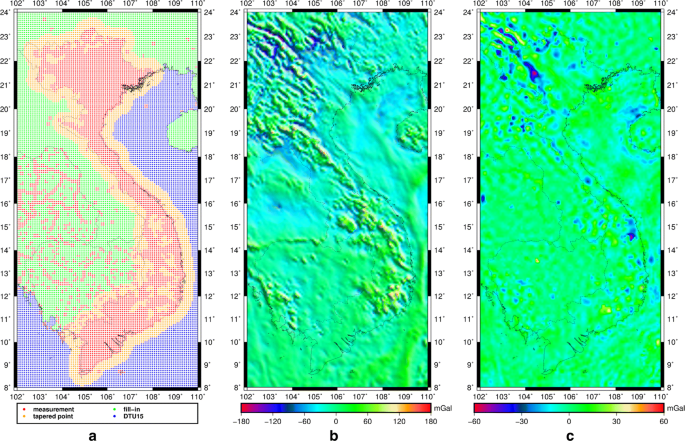

  

  Final gravity data compilation for the study area. a Geographic display of combination of the gravity data: red dots are grid from land gravity points, orange dots are tapered transition points from fill-in data on land or on the sea to land gravity data, and green dots are fill-in points on land and blue dots are DTU15 marine gravity points; b gravity anomalies ∆g_FA; and c grid of residual gravity anomalies

• (3) The transition areas between observations and fill-in models (land transitions starting at the 5′ radius circles to 50 km beyond, coastal transitions starting at the coastline to 50 km on sea) were filled using a combination of data and models.

  From measurement points, the differences between observations and fill-in data were calculated in the following way:

  $$\Delta g_{\mathrm{dif}} = \Delta g_{\mathrm{FA}} - \Delta g_{{{\mathrm{DIR}}/{\mathrm{EGM}}}} |_{2}^{2159} - \Delta g_{\mathrm{RTM}} |_{2160}^{216000}$$

  (7)

  whereas the differences in the fill-in grids (beyond 50 km from the 5′ radius circles) were set to zero. The LSC method in GEOGRID program was then used to interpolate these differences to the transition points ($\Delta g_{\mathrm{dif}}^{\mathrm{grid}}$). Gravity anomalies of transition points were then constructed by adding $\Delta g_{\mathrm{dif}}^{\mathrm{grid}}$ to the fill-in data of transition points as follows:

  $$\Delta g_{\mathrm{trans}}^{\mathrm{grid}} = \Delta g_{{{\mathrm{DIR}}/{\mathrm{EGM}}}} |_{2}^{2159} + \Delta g_{\mathrm{RTM}} |_{2160}^{216000} + \Delta g_{\mathrm{dif}}^{\mathrm{grid}} .$$

  (8)

• (4) For collocation, the actual measurements were used; however, the same fill-in and transition data as in (2) and (3), respectively, were used.

The combination of the heterogeneous gravity data is shown in Fig. 5a. Statistics of the merged gravity anomalies are given in Table 4 and shown in Fig. 5b. These gravity anomalies were reduced using the GGM and RTM effects according to Eq. (3). Table 4 and Fig. 5c show the grid of residual gravity anomalies with three types of gridded data (measurement grid, fill-in grid on land, and DTU on sea) that were merged. These residual gravity anomalies are generally small (< 30 mGal in magnitude). Large residual gravity anomalies occur in mountainous regions (e.g. the northwest and central parts of the study area) where the altitude is greater than 1000 m. The reason for the large residuals is that errors of the DTM and terrestrial gravity in mountainous regions are larger those in flat regions.

Table 4 Statistics of the gravity anomalies and their residuals [Unit: (mGal)]

GNSS/levelling points

From 2009 to 2010, Vietnam Department of Surveying and Cartography carried out GNSS observations on the levelling points. The GNSS baselines were observed using dual-frequency instruments in static mode with a minimum measurement time of 6 h per session. The GNSS data were processed with Bernese software to obtain ellipsoidal heights referred to the WGS84 ellipsoid. The total number of GNSS/levelling stations used in this study is 812, and these are shown in Fig. 6. GNSS/levelling data include horizontal coordinates (latitude, longitude) and the computed height anomaly. Of the 812 GNSS/levelling points, 428 points are first and second order and 384 points are third order of the national levelling networks. First-, second-, and third-order levelling in Vietnam allows misclosure of $5\sqrt {\mathrm{k}}$, $12\sqrt {\mathrm{k}}$, and $25\sqrt {\mathrm{k}}$ mm over a distance of k km, respectively. Normal height is currently used in the national height system of Vietnam. Figure 6 shows that gravity measurements of VIGAC have been made alongside the first- and second-order levelling. The GNSS/levelling geometric height anomalies were compared with those derived from the EGM-DIR-R5 or the mixed DIR/EGM model together with RTM effects. The RTM effect is used as augmentation of GGMs beyond their selected resolution as:

Fig. 6

GNSS/levelling data: yellow dots are first and second order of the national levelling networks, whereas purple dots are third order

$$\Delta \zeta = \zeta^{\mathrm{GNSS/levelling}} - \zeta_{\mathrm{DIR5}} |_{2}^{260} - \zeta_{\mathrm{RTM}} |_{261}^{216000}$$

(9)

$$\Delta \zeta = \zeta^{\mathrm{GNSS/levelling}} - \zeta_{\mathrm{DIR/EGM}} |_{2}^{2159} - \zeta_{\mathrm{RTM}} |_{2160}^{216000}$$

(10)

The results are listed in Table 5. These results clearly show significant improvement (2.5 cm in STD) when using the mixed DIR/EGM instead of using EGM-DIR-R5 only in combination with RTM effects. This demonstrates that EGM2008 performs better than RTM effects computed with TC within the spectral window d/o 260-2159 in Vietnam, even if fill-in data were used.

Table 5 Statistics of the differences between the GNSS/levelling points and the GGM [Unit: (m)]

Quasigeoid model estimation and validation

The residual height anomalies have been determined using the regular grid of residual gravity anomalies employing the Stokes’ integral in the 1D-FFT approach (Haagmans et al. 1993) implemented in the GRAVSOFT SPFOUR program with the Wong–Gore modification (WG) of the Stokes’ kernel function (Wong and Gore 1969). WG removes low harmonics up to degree N₁, so the influence of the local data at long wavelengths is eliminated and then linearly tapered to N₂ (Forsberg and Tscherning 2008). N₁ and N₂ are selected according to data and the GGM used in the remove step, but they should be less than or equal to degree n_max of the GGM. To find out the optimum N₁ and N₂ degree, the quasigeoid was computed by the Stokes FFT using WG with N₁ and N₂ being tested from 100 to 260 (maximum degree of the EGM-DIR-R5 model used in combination with EGM2008) in steps of 10°. The computed quasigeoid models were then compared to GNSS/levelling data. Finally, the best quasigeoid model was obtained when the low harmonics were completely removed from Stokes’ function up to degree N₁ = 220 and then linearly tapered to N₂ = 230.

Residual height anomalies were also calculated with the LSC method, using the GRAVSOFT GEOCOL program. Computation of the empirical and fitted covariance functions of the gravity anomalies is required in LSC to estimate the residual height anomalies. We used the error degree variances of the mixed DIR/EGM model up to 719 and the fourth model of Tscherning and Rapp (1974) for the degree variances of degree > 719. Degree 719 agrees best with the empirical data for fitting the model covariance function. The empirical covariance function of the data has been computed using the GRAVSOFT EMPCOV program and was fitted to the Tscherning and Rapp model using the GRAVSOFT COVFIT program. We have determined the following optimum parameters for inputs of GEOCOL: the depth to the Bjerhammar sphere R − R_B = − 0.028 km and the variance of the gravity anomalies at zero height VARG = 131.06 mGal². Figure 7 shows the plot of the empirical covariance (blue line) and fitted covariance functions for the residual gravity anomalies Δg_res (red line).

Fig. 7

Empirical and fitted covariance functions for residual gravity anomalies Δg_res

The residual height anomalies $\left( {\Delta \zeta_{\mathrm{res}}^{\mathrm{FFT}} } \right)$ computed with the SPFOUR program vary from − 0.701 to 0.402 m. The height anomalies, obtained by restoration of ζ_GGM and ζ_RTM, vary from − 35.097 to 16.684 m (GEOID_FFT solution). The residual height anomalies were also computed with the GEOCOL program: $\Delta \zeta_{\mathrm{res}}^{\mathrm{LSC}}$ varies from − 0.779 to 0.432 m and ζ^LSC from − 34.969 to 16.688 m (GEOID_LSC solution).

Figure 8a, b shows the residual height anomalies $\left( {\Delta \zeta_{\mathrm{res}}^{\mathrm{FFT}} } \right)$ and GEOID_FFT, and the differences between GEOID_FFT and GEOID_LSC are shown in Fig. 8c. The differences range from − 0.232 to 0.244 m. The large differences between GEOID_FFT and GEOID_LSC occur in the regions where the residual gravity anomalies are large (> 30 mGal). This issue will be discussed later.

Fig. 8

Residual height anomalies $\left( {\Delta \zeta_{\mathrm{res}}^{\mathrm{FFT}} } \right)$ (a), GEOID_FFT (b), and difference between GEOID_FFT and GEOID_LSC (c)

For validation, the height anomalies were compared with those inferred from 812 GNSS/levelling reference points (ζ^{GNSS/levelling}). Figure 9a–c shows the plots of the differences of ζ^FFT, ζ^LSC, and ζ^EGM2008 with ζ^{GNSS/levelling}, and the statistics are listed in Table 6. The differences for GEOID_FFT range from 0.136 to 0.816 m with a STD of 0.097 m and average bias of 0.506 m and for GEOID_LSC from 0.138 to 0.815 m with a STD of 0.097 m and average bias of 0.508 m. The results show that both methods reach the same precision, with a STD at the 9.7 cm level. The reason for the large average bias is datum inconsistencies and long wavelength quasigeoid errors. These quasigeoids refer to a global reference system while heights that have been determined from levelling refer to national mean sea level. It should also be noted that here the degree-0 term (e.g. − 41 cm for EGM2008 with the reference ellipsoid WGS84; http://earth-info.nga.mil/GandG/wgs84/gravitymod/egm2008/egm08_wgs84.html) is not included in this average bias. The results of the comparison indicated significant improvement in the local quasigeoids over EGM2008 and EIGEN-6C4 in Vietnam, which have STD of 29.1 and 19.2 cm, respectively. Figure 9 shows this improvement over EGM2008, especially in the north and the mountainous regions.

Fig. 9

Differences between the developed quasigeoid and GNSS/levelling. a GEOID_FFT, b GEOID_LSC, and c EGM2008

Table 6 Statistics of the quasigeoid and their validation with GNSS/levelling data [Unit: m]

We have also compared these quasigeoids with GNSS/levelling points split according to order: 428 points of first- and second-order levelling and 384 points of third-order levelling. The results of GEOID_LSC show a STD of 8.7 cm for the first- and second-order points (where gravity was measured) and 10.8 cm for the third-order points (where gravity was not measured), while GEOID_FFT has a STD of 9.1 cm for the first- and second-order points and 10.4 cm for the third-order points (Table 7). These results show that the LSC method is a little more precise than the 1D FFT where gravity data are available. To further clarify this issue, we have evaluated the quasigeoid in two areas (two rectangles in Fig. 3) where there is sufficient terrestrial gravity as well as GNSS/levelling data (136 GNSS/levelling points in a northern area defined by 20° ≤ φ ≤ 22° in latitude and 105° ≤ λ ≤ 108° in longitude and 120 GNSS/levelling points in a southern area defined by 8° ≤ φ ≤ 11° in latitude and 104° ≤ λ ≤ 108° in longitude). For the northern area, the STD of the LSC and 1D FFT methods is 7.4 cm and 8.2 cm, respectively; for the southern area, the STDs are 9.2 cm and 10.0 cm, respectively. The results of the comparison indicated that the LSC method is more precise than the 1D FFT method, 0.8 cm of STD for each area. However, quality of the available gravity data in Vietnam is not homogeneous (bias, precision between IGP, VIGAC, and fill-in data) and not enough information on the accuracy is available, which is challenging with the LSC method while with the Stokes FFT method a good data density is required. It is the reason why these two methods have the same accuracy for the whole study area. The circles in Figs. 8c, 9a, b show the area where the difference between the two quasigeoid solutions is significant (and where terrestrial gravity data is available). The higher accuracy of LSC, which uses all observations, may be due to the higher density of measurements in these areas than for other areas; a denser residual gravity grid could have been computed for SPFOUR. This hypothesis was confirmed by computing and using denser grids (2.5′ × 2.5′) for the two test areas with the Stokes FFT method. The results are shown in the last 2 rows in Table 7, and they indicate that the Stokes FFT method has the same accuracy as the LSC method over these two areas when GEOID_FFT is computed with the denser grids.

Table 7 Differences between the quasigeoid and GNSS/levelling data according to the order of levelling network [Unit: m]

The STD of the differences between EGM2008 and EIGEN-6C4 with 384 GNSS/levelling points of the third-order levelling is 27.4 cm and 18.6 cm (Table 7), respectively, whereas the STD of GEOID_FFT and GEOID_LSC is 10.8 and 10.4 cm, respectively. These numerical findings signify that the addition of the RTM effects to DIR/EGM has significantly improved the accuracy of the height anomalies in the area where no data existed.

Moreover, a quasigeoid was computed using DTU15 data (ζ^FFT-DTU) instead of using the mixed DIR/EGM model together with RTM effect within 50 km from the coastline. The height anomalies derived from these quasigeoids were compared with those derived from 69 GNSS/levelling points near the coast (ζ^{GNSS/levelling_coast} in Table 7). An improvement can be seen when using RTM effects together with the mixed DIR/EGM model instead of using DTU15 gravity within 50 km from the coastline. This suggests that RTM effects together with the DIR/EGM model can be used to fill the gap between gravity data on land and marine altimetric gravity if airborne or shipborne gravity is not available in coastal zones.

To assess the applicability of the developed quasigeoid model in GNSS levelling, a test was performed in a relative sense. The relative fits of GEOID_LSC to GNSS/levelling data were determined over 21,161 baselines (baseline length < 100 km). Figure 10a, b shows the discrepancies between height anomaly differences derived from EGM2008 (d/o 2190) and GEOID_LSC with those derived from GNSS/levelling data. The tolerance of fourth-order spirit levelling was used for verification. With GEOID_LSC, 19,237 (90.91%) baselines comply, while with EGM2008 only 10,158 (52.00%) baselines do. With EGM2008, the accuracy of GNSS levelling cannot reach fourth-order levelling requirements. With GEOID_LSC, there are still 1924 baselines that lie outside the tolerance of fourth-order levelling, probably due to errors in GNSS/levelling data; error detection methods must be applied to clean the GNSS/levelling data before fitting with a gravimetric quasigeoid. Moreover, a large bias was also found between gravimetric quasigeoid and GNSS/levelling data (50 cm) in which the degree-0 term also needs to be taken into account to determine the true vertical datum offsets for Vietnam with respect to a global equipotential surface. Such offsets must be corrected for before using a quasigeoid in GNSS levelling. These issues will be solved in future research. Figure 10c shows the discrepancies between height anomaly differences derived from GEOID_LSC and those derived from GNSS/levelling data in the northern test area (defined by 20.5° ≤ φ ≤ 21.5° in latitude and 106° ≤ λ ≤ 107.5° in longitude), but with the tolerance set by third-order spirit levelling ($12\sqrt {\mathrm{k}}$ mm over a distance of k km was used to compare). There are 201 (81.05%) baselines (over a total of 248 baselines) that lie inside the tolerance of third-order levelling. We also tested for the southern area (defined by 11° ≤ φ ≤ 12° in latitude and 106° ≤ λ ≤ 108.5° in longitude); there are 172 (78.89%) baselines (over a total of 218 baselines) that lie inside this tolerance. This suggests that with gravity data for the entire country of similar quality and distribution as for these areas, the resulting quasigeoid may allow GNSS levelling to comply with third-order levelling specifications.

Fig. 10

Magnitude of relative differences between EGM2008 (d/o 2190) and GEOID_LSC with GNSS/levelling data over 21,161 baselines (blue), fourth-order tolerance (orange), a EGM2008, b GEOID_FFT, and c magnitude of relative differences between GEOID_LSC and GNSS/first- and second-order levelling data in north area over 248 baselines (blue), third-order tolerance (green)

Conclusions

A new quasigeoid model has been generated for Vietnam and surrounding areas from the combination of heterogeneous data including 29,121 terrestrial gravity points, global gravity models, and high-resolution topographic and bathymetric data. Two gravimetric quasigeoid solutions, called GEOID_FFT and GEOID_LSC, were computed with the Stokes’ integral using the FFT-1D approach and deterministic kernel modification as proposed by Wong–Gore and the LSC method, respectively. These quasigeoid models were validated through a comparison with 812 GNSS/levelling points. Our results show that both models lead to very similar results reaching a STD at the 9.7 cm level with a mean bias of 50 cm. The results of the comparison indicated significant improvement in these models over the commonly used EGM2008 and EIGEN-6C4 for Vietnam in all areas, covered or not by land gravity measurements. Such regional models are thus likely to be used for GNSS levelling applications, with accuracy satisfying fourth-order levelling for the entire country and third order in areas where there are sufficient data (north and south areas), and should also contribute to the modernization of Vietnam’s height system. A significant improvement for areas with poor data coverage proves that the recent GOCE/GRACE GGM in combination with EGM2008 and RTM effects may be used to improve quasigeoid determination in the areas where gravity data are not available or insufficient, especially in mountainous regions and coastal zones. The best agreement in Vietnam is observed for EGM-DIR-R5 used up to d/o 260, EGM2008 used up from d/o 270 to 2159 and RTM effects used equivalent to d/o 216000.

Land gravity data are not available for large parts of the mountainous region, and consequently, the gravimetric quasigeoid solutions are significantly less accurate there. Improvement in the proposed quasigeoid model will require better data coverage over land and sea in Vietnam and its vicinity. These regions have to be covered with preferentially airborne data and shipborne data.

References

Andersen OB, Knudsen P (2016). Deriving the DTU15 Global high resolution marine gravity field from satellite altimetry. In: ESA Living Planet Symposium 2016, Prague, Czech Republic, 5–13 May 2016
Balmino G, Lambeck K, Kaula WM (1973) A spherical harmonic analysis of the Earth’s topography. J Geophys Res 78:478–481. https://doi.org/10.1029/JB078i002p00478
Balmino G, Vales N, Bonvalot S, Briais A (2012) Spherical harmonic modelling to ultra-high degree of Bouguer and isostatic anomalies. J Geod 86:499–520. https://doi.org/10.1007/s00190-011-0533-4
Becker JJ, Sandwell DT, Smith WHF et al (2009) Global bathymetry and elevation data at 30 arc seconds resolution: SRTM30_PLUS. Mar Geod 32:355–371. https://doi.org/10.1080/01490410903297766
Bonvalot S (2016) BGI—The International Gravimetric Bureau. In “The Geodesist’s Handbook 2016”. J Geod 90:907–1205. https://doi.org/10.1007/s00190-016-0948-z
Brockmann JM, Zehentner N, Höck E et al (2014) EGM_TIM_RL05: an independent geoid with centimeter accuracy purely based on the GOCE mission. Geophys Res Lett 41:8089–8099. https://doi.org/10.1002/2014GL061904
Bruinsma SL, Förste C, Abrikosov O et al (2014) ESA’s satellite-only gravity field model via the direct approach based on all GOCE data. Geophys Res Lett 41:7508–7514. https://doi.org/10.1002/2014GL062045
Denker H (2005) Evaluation of SRTM3 and GTOPO30 terrain data in Germany. In: Jekeli C, Bastos L, Fernandes J (eds) Gravity, geoid and space missions. Springer, Berlin, pp 218–223
Drinkwater MR, Floberghagen R, Haagmans R et al (2003) GOCE: ESA’s first earth explorer core mission. In: Beutler G, Drinkwater MR, Rummel R, Von Steiger R (eds) Earth gravity field from space—from sensors to earth sciences. Space sciences series of ISSI, vol 18. Kluwer Academic Publishers, Dordrecht, Nertherlands, pp 419-432 (ISBN: 1-420-1408-2)
Dumrongchai P, Wichienchareon C, Promtong C (2012) Local geoid modeling for Thailand. Int J Geoinform 8(4):15–26
Ekman M (1989) Impacts of geodynamic phenomena on systems for height and gravity. Bull Geodesique 63:281–296. https://doi.org/10.1007/BF02520477
Farr TG, Rosen PA, Caro E et al (2007) The shuttle radar topography mission. Rev Geophys. https://doi.org/10.1029/2005rg000183
Featherstone WE (2010) Satellite and airborne gravimetry: their role in geoid determination and some suggestions. In: Lane R (ed) Airborne gravity 2010. Geoscience Australia, Canberra
Featherstone WE, Kirby JF, Kearsley AHW et al (2001) The AUSGeoid98 geoid model of Australia: data treatment, computations and comparisons with GPS-levelling data. J Geod 75:313–330. https://doi.org/10.1007/s001900100177
Featherstone WE, Kirby JF, Hirt C et al (2011) The AUSGeoid09 model of the Australian Height Datum. J Geod 85:133–150. https://doi.org/10.1007/s00190-010-0422-2
Final Report: Measurement and Improvement of Vietnam National Gravity Data (2012). Vietnam Institute of Geodesy and Cartography (VIGAC)
Forsberg R (1984) A study of terrain reductions, density anomalies and geophysical inversion methods in gravity field modeling. Scientific Report No. 5, Department of Geodetic Science and Surveying, Ohio State University, Colombus, Ohio, USA
Forsberg R, Olesen AV (2010) Airborne gravity field determination. In: Xu G (ed) Sciences of Geodesy—I. Springer, Berlin, Heidelberg, pp 83–104. https://doi.org/10.1007/978-3-642-11741-1_3
Forsberg R, Tscherning CC (2008) An overview manual for the GRAVSOFT geodetic gravity field modelling programs, 2nd edn, DTU Space. http://cct.gfy.ku.dk/publ_cct/cct1936.pdf
Forsberg R, Olesen AV, Einarsson I et al (2014a) Geoid of Nepal from airborne gravity survey. In: Rizos C, Willis P (eds) Earth on the edge: science for a sustainable planet. Springer, Berlin, pp 521–527
Forsberg R, Olesen AV, Gatchalian R, Ortiz CCC (2014b) Geoid model of the Philippines from airborne and surface gravity. National Mapping and Resource Information Authority
Förste C, Bruinsma SL, Abrikosov O, et al (2014) EIGEN-6C4 the latest combined global gravity field model including GOCE data up to degree and order 2190 of GFZ Potsdam and GRGS Toulouse. GFZ Data Services. http://doi.org/10.5880/icgem.2015.1
Gatchalian R, Forsberg R, Olesen A (2016) PGM2016: a new geoid model for the Philippines. Report of National Mapping and Resource Information Authority (NAMRIA), Dept. of Environmental and Natural Resources, Republic of The Philippines
Gatti A, Reguzzoni M, Migliaccio F, Sansò F (2016) Computation and assessment of the fifth release of the GOCE-only space-wise solution. In: ResearchGate. https://www.researchgate.net/publication/316042680_Computation_and_assessment_of_the_fifth_release_of_the_GOCE-only_space-wise_solution. Accessed 27 Nov 2018
Gilardoni M, Reguzzoni M, Sampietro D, Sanso F (2013) Combining EGM2008 with GOCE gravity models. Bollettino di Geofisica Teorica ed Applicata 54(4):285–302. https://doi.org/10.4430/bgta0107
Haagmans R, de Min E, van Gelderen M (1993) Fast evaluation of convolution integrals on the sphere using 1-D FFT, and a comparison with existing methods for Stokes’ integral. Manuscripta Geodaetica 18:227–241
Hirt C (2013) RTM gravity forward-modeling using topography/bathymetry data to improve high-degree global geopotential models in the coastal zone. Mar Geod 36:183–202. https://doi.org/10.1080/01490419.2013.779334
Hofmann-Wellenhof B, Moritz H (2006) Physical Geodesy, 2nd edn. Springer-Verlag, Wien
Ismail MK, Din AHM, Uti MN, Omar AH (2018) Establishment of new fitted geoid model in Universiti Teknologi Malaysia. In: ResearchGate. https://www.researchgate.net/publication/328683742_Establishment of new fitted geoid model in Universiti Teknologi Malaysia. Accessed 22 Nov 2018
Jamil H, Kadir M, Forsberg R et al (2017) Airborne geoid mapping of land and sea areas of East Malaysia. J Geod Sci 7:84–93. https://doi.org/10.1515/jogs-2017-0010
Kuroishi Y, Ando H, Fukuda Y (2002) A new hybrid geoid model for Japan, GSIGEO2000. J Geod 76:428–436. https://doi.org/10.1007/s00190-002-0266-5
Lee SB, Auh SC, Seo DY (2017) Evaluation of global and regional geoid models in South Korea by using terrestrial and GNSS data. KSCE J Civ Eng 21:1905–1911. https://doi.org/10.1007/s12205-016-1096-y
Lemoine FG, Kenyon SC, Factor JK et al (1998) The development of the joint NASA GSFC and the National Imagery and Mapping Agency (NIMA) geopotential model EGM96. NASA Goddard Space Flight Center, Greenbelt, Maryland, USA
Mayer-Guerr T (2015) The combined satellite gravity field model GOCO05s. Presentation at EGU General Assembly 2015, id.12364, Vienna, Austria, 12-17 April 2015
Miyahara B, Kodama T, Kuroishi Y (2014) Development of new hybrid geoid model for Japan, “GSIGEO2011”. Bull Geogr Inf Authority Japan 62:11–20
Pail R, Fecher T, Barnes D et al (2018) Short note: the experimental geopotential model XGM2016. J Geod 92:443–451. https://doi.org/10.1007/s00190-017-1070-6
Pavlis NK, Holmes SA, Kenyon SC, Factor JK (2012) The development and evaluation of the Earth Gravitational Model 2008 (EGM2008). J Geophys Res Solid Earth. https://doi.org/10.1029/2011jb008916
Piñón DA, Zhang K, Wu S, Cimbaro SR (2018) A new argentinean gravimetric geoid model: GEOIDEAR. In: Freymueller JT, Sánchez L (eds) International symposium on earth and environmental sciences for future generations. Springer International Publishing, pp 53–62
Rapp RH (1989) The treatment of permanent tidal effects in the analysis of satellite altimeter data for sea surface topography. Manuscripta Geodetica 14(6):368–372
Sansò F, Sideris MG (eds) (2013) Geoid determination: theory and methods. Springe, Berlin
Torge W, Müller J (2012) Geodesy, 4th edn. De Gruyter, Berlin
Tscherning CC, Rapp RH (1974) Closed covariance expressions for gravity anomalies, geoid undulations, and deflections of the vertical implied by anomaly degree variance models. Accessed 28 June 2018
Wessel P, Smith WHF (1998) New, improved version of generic mapping tools released. EOS Trans Am Geophys Union 79(47):579. https://doi.org/10.1029/98EO00426
Wong L, Gore R (1969) Accuracy of geoid heights from modified stokes kernels. Geophys J R Astron Soc 18:81–91. https://doi.org/10.1111/j.1365-246X.1969.tb00264.x
Yun H-S (2002) Evaluation of ultra-high and high degree geopotential models for improving the KGEOID98. Korean J Geomat 2:7–15
Acknowledgements
We are very grateful to the VIGAC, IGP-VAST, and BGI (http://bgi.obs-mip.fr/) that supplied data for this study. This study was also supported by CNES. The authors would like to thank the authors of GRAVSOFT (DTU) for providing their software. The SRTM3arc_v4.1 is available via http://srtm.csi.cgiar.org/SELECTION/inputCoord.asp. The SRTM15arc_plus model is available via https://topex.ucsd.edu/pub/srtm15_plus/. All used GGMs in this paper are available via http://icgem.gfz-potsdam.de/tom_longtime. The DTU15 gravity is available via https://ftp.space.dtu.dk/pub/. In this paper, we used the Generic Mapping Tools (GMT) for producing some of figures. We thank the anonymous reviewers for their constructive comments and helpful suggestions.
Funding
Dinh Toan VU receives funding of the Vietnamese Government’s 911 project and University Paul Sabatier (UPS)-GET. This study is also supported by CNES.
Author information
Authors and Affiliations
Contributions
DTV performed all the data processing and drafted the manuscript. All authors analysed and discussed the preliminary results. SB and SB provided critical comments for this study and supported the observations. All authors read and approved the final manuscript.
Corresponding author
Ethics declarations
Competing interests
The authors declare that they have no competing interests.
Additional information
Publisher's Note
Springer Nature remains neutral with regard to jurisdictional claims in published maps and institutional affiliations.
Rights and permissions
Open Access This article is distributed under the terms of the Creative Commons Attribution 4.0 International License (http://creativecommons.org/licenses/by/4.0/), which permits unrestricted use, distribution, and reproduction in any medium, provided you give appropriate credit to the original author(s) and the source, provide a link to the Creative Commons license, and indicate if changes were made.
About this article
Cite this article
Vu, D.T., Bruinsma, S. & Bonvalot, S. A high-resolution gravimetric quasigeoid model for Vietnam. Earth Planets Space 71, 65 (2019). https://doi.org/10.1186/s40623-019-1045-3
Received:
Accepted:
Published:
DOI: https://doi.org/10.1186/s40623-019-1045-3