- Full paper
- Open access
- Published:
The development and validation of a ‘flux-corrected transport’ based solution methodology for the plasmasphere refilling problem following geomagnetic storms
Earth, Planets and Space volume 72, Article number: 26 (2020)
Abstract
The refilling of the plasmasphere following geomagnetic storms remains one of the longstanding and interesting problems in ionosphere–magnetosphere coupling research. The objective of this paper is the formulation and development of a one-dimensional (1D) refilling model using the flux-corrected transport method, a numerical method that is well-suited to handling problems with shocks and discontinuities. In this paper, the developed methodology has been validated against exact, analytical benchmarks, and good agreement has been obtained between these analytical benchmarks and numerical results. The objective of this research is the development of a three-dimensional (3D) multi-ion model for ionosphere–magnetosphere coupling problems in open and closed line geometries.

Introduction
The refilling of the plasmasphere following a geomagnetic storm remains one of the longstanding and interesting problems in ionosphere–magnetosphere coupling research. (Banks et al. 1971; Carpenter and Park 1973; Darrouzet et al. 2009; Goldstein et al. 2002; Gringauz 1963; Millian and Thorne 2007; Obana et al. 2019; Pezzopane et al. 2019; Sandel et al. 2003) As a direct effect of a geomagnetic storm, the plasma in the outer boundaries of the plasmasphere is removed from the region by storm-time electric fields and convected to the magnetopause in the sunward direction. Thus, the plasma contained inside the magnetic flux tubes is lost, and at the end of the geomagnetic storm, the outer layers of the plasmasphere are significantly depleted. The pressure gradient between the ionosphere and the depleted outer plasmasphere drives the ionospheric plasma upward along the magnetic flux tubes, which initiates the refilling process.
The primary focus of this work is the development of a hydrodynamic model geared toward the numerical solution of the refilling problem, along with the development of benchmarks for its validation. A schematic diagram of the flux tube at the end of the geomagnetic storm is shown in Fig. 1.

The schematic of a flux tube after a geomagnetic storm, where the ionosphere is shown by hatched lines. The depleted flux tube lies above the ionosphere. The symbols θ and r represent colatitude and geocentric distance, respectively, and S =+ Smax show the boundaries in the conjugate ionospheres (Singh et al. 1986; Rasmussen and Schunk 1988)
During the last several decades, several numerical studies have been undertaken to model plasma transport between the ionosphere and the plasmasphere and these studies have led to the development of ionosphere–magnetosphere coupling models. These models can be divided into two broad categories. In the first category of models (called ‘diffusion models’), the nonlinear inertial terms in the plasma transport equations are ignored, and thus, these models are limited to low-speed diffusion dominated flows. This category of models includes the Sheffield University Plasmasphere Ionosphere Model (SUPIM) (Bailey et al. 1997), the Ionosphere–Plasmasphere Model (IPM) (Schunk et al. 2004), and the Field-Line Interhemispheric Plasma (FLIP) model (Young et al. 1980). The FLIP model has recently been integrated into the Ionosphere Plasmasphere Electrodynamics (IPE) model and a different category of models that exists in the literature, where the nonlinear inertial terms are retained in the transport equations, is the so-called ‘hydrodynamic model,’ introduced by Banks et al. (1971) and further developed by Khazanov et al. (1984), Singh et al. (1986) and Rasmussen and Schunk (1988). Based on our literature survey, as of today, the most well-developed hydrodynamic model of the low-latitude ionosphere is SAMI2/SAMI3 introduced by Huba and Joyce (2000) and later applied to ionosphere–magnetosphere coupling (Krall and Huba 2013, 2019) problems. In this model, the motion along the field line is described by a set of advection/diffusion equations, and these equations are solved using the implicit donor cell method (Hoffmann and Chiang 2000), which is first-order in nature.
In this paper, we present a ‘flux-corrected transport’ (FCT) based solution methodology (Boris and Book 1976; Kuzmin et al. 2012), a method that is accurate to second-order which provides the scientific rationale for adapting the method to ionospheric outflow problems. FCT-based solution methodologies have been developed for the plasmasphere refilling problem for a single (H+) ion (Singh et al. 1986; Rasmussen and Schunk 1988), where neither the algorithmic details nor the validating benchmarks were presented. In Chatterjee’s doctoral dissertation (Chatterjee 2018), an FCT-based solution methodology was developed independently of Singh et al. (1986) and Rasmussen and Schunk (1988), and this solution methodology has the capability of accommodating multiple ions and neutrals. The refilling results involving multiple ions and neutrals are presented in Chatterjee (2018) and Chatterjee and Schunk (2019), but here in this paper, the basic algorithmic details of the solution methodology developed in Chatterjee (2018) are provided along with the validating analytical benchmarks that are close approximations of the refilling problem. The validation benchmarks and results described in the following sections involve only H+ ions.
A brief description of the FCT-based solution methodology
In this section, the plasmasphere refilling problem is modeled as a single ion species (\({\text{H}}^{ + }\) ions) along with electrons and refilling along a 1D flux tube, without considering the curvature of the tube and neglecting the effects from Coulomb collisions. The time-dependent continuity and momentum equations are given below (Oran and Boris 2001):
where t is time, x the spatial coordinate, \(n_{i,e}\) the ion/electron concentration, \(u_{i,e}\) ion/electron velocity, \(m_{i,e}\) the ion/electron mass, \(p_{i,e} = n_{i,e} kT\) the partial ion/electron pressure, T the constant temperature along the flux tube, k the Boltzmann constant, E the electric field and \(g\left( x \right)\) the spatially dependent gravitational force. Imposing quasi-neutrality gives rise to \(n_{i} = n_{e}\) and neglecting the electron mass in the electron momentum equation gives rise to an expression for the electric field given by \(E = - \left( {kT/en_{i} } \right)\left( {\partial n_{i} /\partial x} \right)\). The substitution of this electric field in the ion momentum equation gives rise to the set of equations given by
and this set of equations is solved using the FCT method (Boris and Book 1976; Kuzmin et al. 2012). The specific scheme adopted in this work is a generalization of Otto (2013). In Otto (2013), the source terms were assumed to be zero, but in the solution methodology that we have developed, non-zero source terms can be accommodated.
We re-write Eq. (2) as
From a numerical standpoint, the difficulty lies in the fact that immediately after a geomagnetic storm, there is a sharp discontinuity at the ionosphere–plasmasphere boundary. Had it not been for this discontinuity, a second-order scheme such as the Lax–Wendroff (MacCormack method) would have been adequate, where the numerical method itself does not introduce any diffusion in the problem (Hoffmann and Chiang 2000). The fundamental philosophy behind flux-correction is that “diffusion” is artificially introduced at spatial points where shocks and discontinuities are present. To formulate a flux-correction based solution, a solution based on the Lax–Wendroff (MacCormack method) scheme denoted as \(f_{i}^{{k,{\text{LW}}}} ,\) is first introduced, where the subscript i represents the spatial index and the superscript k represents the time index. The Lax–Wendroff scheme is a two-step scheme given by
In the flux-corrected scheme adopted in this work, a diffusive flux is generated after the first step using
while an anti-diffusive flux is generated after the second step and defined as follows
There can be many choices for the diffusion and anti-diffusion coefficients, but a widely used choice (Otto 2013) is given below
with \(\alpha_{0} = 1/6,\alpha_{1} = 1/3,\alpha_{2} = - 1/6.\) The solution with diffusion introduced into it can now be computed using
and the variation in the diffusive solution between successive grid points is computed as
As mentioned before, the fundamental premise of flux-correction is that diffusion is not required at points in space where the solution is continuous and smooth. As a result, the anti-diffusive flux is modified by comparing the variation in the diffusive solution given by Eq. (9) with the anti-diffusive flux \(\varvec{P}_{i + 1/2}^{{k,{\text{AD}}}}\) given by Eq. (6):
where \(\sigma_{i + 1/2} = {\text{sgn}}\left( {\varvec{P}_{i + 1/2}^{{k,{\text{AD}}}} } \right)\). Finally, the modified anti-diffusive flux is applied to the solution; it mitigates the effects of unnecessary diffusion and the flux-corrected solution for Eq. (3) is given by
Discussion of results
The results for three benchmark applications are given below:
- A.
The problem of the propagation of a wave with a constant velocity in an 1D problem domain is considered, which is the equivalent of solving mass transport under the approximation of constant drift velocity:
$$\frac{\partial n}{\partial t} = - u\frac{\partial n}{\partial x},u > 0,n\left( {x,0} \right) = f\left( x \right),n\left( {x,t} \right) = f\left( {x - ut} \right) ,$$(12)where n is the propagating quantity of interest (say concentration), x the position coordinate, t time, u the constant wave/drift velocity and f(x) any given initial condition. However, if the initial condition is a function with spatial discontinuities, such as the square wave, a second-order scheme such as Lax–Wendroff given in Eq. (4) produces spatial oscillations as shown in Fig. 2a. It should be noted that this kind of spatial discontinuities is indeed encountered in the plasmasphere refilling problem.
Fig. 2 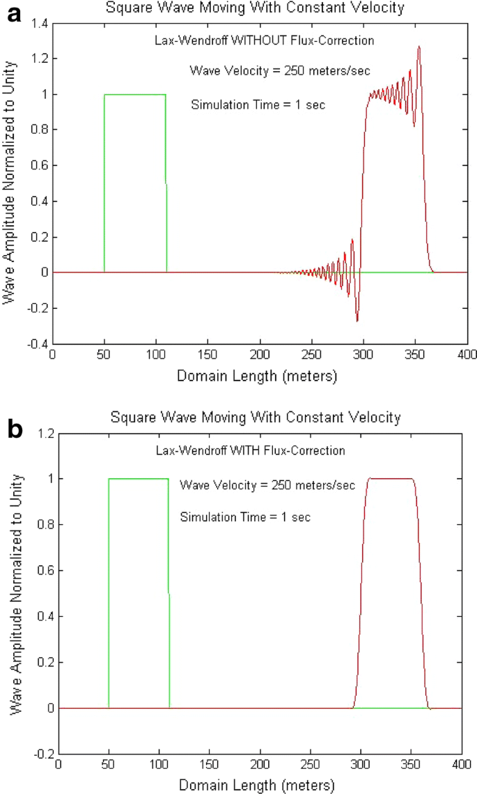
a Square wave propagation without flux-correction. A square wave with constant amplitude propagating through a 1D problem domain: Lax–Wendroff scheme without flux-correction. The initial square wave is given in green; the square wave after 1 s is given in red. The fluctuations on the edges arise from the discontinuity in the initial square wave at the edges and the use of a second-order algorithm. b Square wave propagation with flux-correction. A square wave with constant amplitude propagating through 1D problem domain: Lax–Wendroff scheme with flux-correction. The initial square wave is given in green; the square wave after 1 s is given in red. The fluctuations on the edges observed in a are eliminated by use of flux-correction
This problem of spatial oscillations is easily mitigated using the flux-corrected scheme described in Eqs. (3)–(11), and the results are shown in Fig. 2b. As expected, flux-correction was able to remedy the problem of oscillation at the edges, but at the expense of the broadening of the solution resulting from the introduction of diffusion, which begs the question if the flux-corrected method can provide the required level of accuracy for the plasmasphere refilling problem. With that in mind, a problem similar in spirit to the refilling problem for which an analytical solution exists is chosen as Benchmark Problem B.
- B.
The problem in Eq. (1) is simplified by ignoring the contribution from the gravitational force and the result is isothermal plasma expanding into vacuum. The specifics of the problem and solution to this problem are given in Eq. (13). In this problem, a constant, sub-sonic drift velocity is imposed on the plasma, and this is a generalization of the self-similar solution in Schunk and Nagy (2009) where the initial velocity of the plasma was zero:
$$\begin{aligned} & \frac{{\partial \varvec{n}}}{\partial t} + \frac{{\partial \varvec{P}}}{\partial x} = 0,\varvec{n} = \left\{ {\begin{array}{*{20}c} n \\ {nu} \\ \end{array} } \right\},\varvec{P} = \left\{ {\begin{array}{*{20}c} {nu} \\ {p/m + nu^{2} } \\ \end{array} } \right\} \\ & x \le 0:n\left( {x,0} \right) = n_{0} ,u\left( {x,0} \right) = u_{0} \\ & x > 0:n\left( {x,0} \right) = 0,u\left( {x,0} \right) = 0 \\ & x \le \left( {u_{0} - u_{\text{th}} } \right)t: n\left( {x,t} \right) = n_{0} ,u\left( {x,t} \right) = u_{0} \\ & x > \left( {u_{0} - u_{\text{th}} } \right)t:n\left( {x,t} \right) = n_{0} e^{{ - \left( {\xi - \frac{{u_{0} }}{{u_{\text{th}} }} + 1} \right)}} ,u\left( {x,t} \right) = u_{\text{th}} \left( {\xi + 1} \right) \\ \end{aligned}$$(13)where \(u_{\text{th}} = \sqrt {kT/m}\) is the ion-acoustic speed and \(\xi = \left( {x/tu_{\text{th}} } \right)\) is known as the self-similar parameter. The solution is characterized by a “rarefaction” wave moving back into the plasma layer with the ion-acoustic speed, and it can be observed from Fig. 3a, b that there is excellent agreement between the numerical solutions and the analytical results. The self-similar solution captures the essence of the refilling problem at its onset after a magnetic storm when the concentration of the ions is small inside the plasmasphere. Thus, the concentration gradient is large at the ionosphere–plasmasphere boundary, thus making the sum of the pressure gradient and electric field term in Eq. (1) significantly greater than the gravitational force term.
Fig. 3 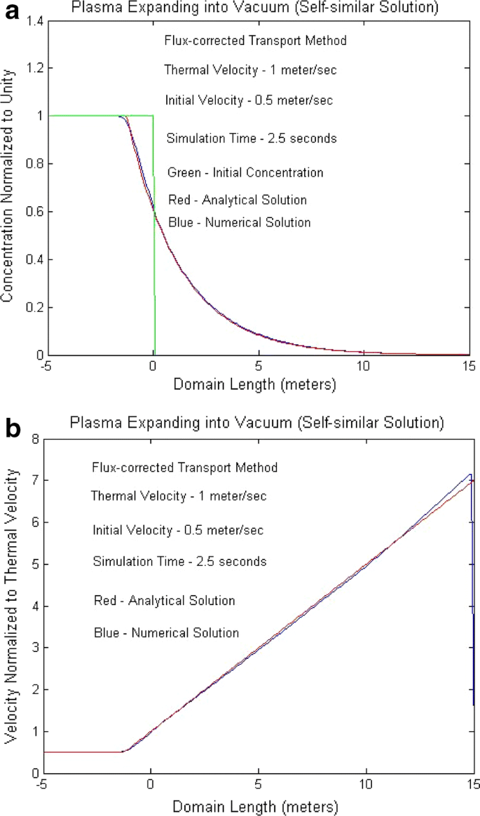
a Concentration profile showing plasma escaping into vacuum. Other than the concentration gradient, the plasma has an initial drift velocity. The initial concentration is shown in green, the analytical solution (after a given interval of time) is shown in red and the numerical solution (after the same interval of time) is shown in blue. b Velocity profile showing plasma escaping into vacuum. Other than the concentration gradient, the plasma has an initial drift velocity. The initial concentration is shown in green, the analytical solution (after a given interval of time) is shown in red and the numerical solution is shown in blue
- C.
In the third application example, plasmasphere refilling after a geomagnetic storm is modeled as a single-stream isothermal flow of \({\text{H}}^{ + }\) ions, governed by mass and momentum conservation equations. The standard collision-dominated energy conservation equation is not rigorously valid in the plasmasphere and our eventual objective is to replace the constant temperature in our model with a spatially varying temperature profile from an empirical model (Titheridge 1998), which has been seen to produce results more consistent with experiments when it was integrated into the IPM (Schunk et al. 2004). In this problem, the position coordinate in Eq. (2) lies within the range \(0 \le x \le X,\) where X = 58,000 km is the length of the L =4 magnetic field line. It is assumed that plasma expands into the simulation domain at both ends (x = 0 and x = X). It is also assumed that gravity opposes the inward plasma expansion, so gravity points to the right on one side of the equator and to the left on the other side of the equator. A constant temperature of 3560 K is assumed for both electrons and ions, which corresponds to an ion-acoustic speed \(\left( {u_{\text{th}} } \right)\) of 5.4 km/s. A constant gravitational force is assumed over the entire field line, which is the average of the gravitational force at the equator and at either extremity of the field line:
$$\begin{aligned} & g\left( x \right) = - g^{\prime } ,0 \le x < 0.5X \\ & g\left( x \right) = 0,x = 0.5Xg\left( x \right) = g^{\prime } ,0.5X < x \le X, \\ \end{aligned}$$(14)where \(g^{\prime}\) = 2.45 m/s2. The boundary conditions imposed for the concentration and velocity of \({\text{H}}^{ + }\) ions are given by
$$n_{i} \left( {0,t} \right) = n_{0} , n_{i} \left( {X,t} \right) = n_{0} , u_{i} \left( {0,t} \right) = 2\,{\text{km}}/{\text{s}}, u_{i} \left( {X,t} \right) = - 2\,{\text{km}}/{\text{s}}$$(15)where \(n_{0}\) is the concentration at the extremities of the flux tube. The constant gravitational force given in Eq. (14) and the boundary conditions given by Eq. (15) give rise to a steady-state solution given by
$$\begin{aligned} & n_{i}^{s} = n_{0} e^{{ - g^{\prime}x/2u_{\text{th}}^{2} }} ,0 < x < 0.5Xn_{i}^{s} = n_{0} e^{{g^{\prime}\left( {x - X} \right)/2u_{\text{th}}^{2} }} ,0.5X < x < X \\ & u_{i}^{s} = 0,0 < x < X \\ \end{aligned}$$(16)which is obtained by setting \(\partial n_{i} /\partial t,\partial u_{i} /\partial t\) and \(\partial u_{i} /\partial x\) equals to zero in Eq. (2). The initial conditions on \(n_{i}\) and \(u_{i}\) are assumed to be
$$\begin{aligned} & 0 < x < X \\ & n_{i} \left( {x,0} \right) = 0, u_{i} \left( {x,0} \right) = 0. \\ \end{aligned}$$(17)


In general, the imposition of boundary conditions in numerical models (Oran and Boris 2001) can be implemented in three different ways:
- A.
The unknown variables are formulated as linear superpositions of expansion functions where the boundary conditions are satisfied automatically. The method of flux-correction cannot be applied systematically to algorithms that use expansions.
- B.
The second approach is to develop separate finite-difference formulas for boundary cell values in addition to finite-difference formulas developed for points in the interior of the problem domain. This approach can be easy or difficult depending on the complexity of the problem and/or the boundary conditions.
- C.
The third approach is to develop extrapolations from ghost or guard cells that extend outside the computational domain outside the domain boundary. The cells on the domain boundaries are treated as interior cells and of the three methods; this is the easiest and most flexible.
In our problem, the boundary conditions of interest in Eq. (15) are imposed on the external guard cells. At small time scales, at the onset of refilling, the concentration gradient term in Eq. (2) dominates the gravitational force term. As a result, the concentration and velocity profiles after 10 min, shown in Fig. 4a, b, are qualitatively similar to the solution profiles shown in Fig. 3a, b, respectively, and the maximum refilling velocity reaches a value greater than 25 km/s. This value is consistent with numbers reported in the literature (Singh et al. 1986; Rasmussen and Schunk 1988).

a Hydrogen ion concentration profile after 10 min. The concentration normalized to the concentration at the base altitude is imposed on the guard cells. The drift velocity normalized to the hydrogen thermal velocity is imposed on the guard cells. The domain length is normalized to the length of the flux tube. b Hydrogen ion velocity profile after 10 min. The concentration normalized to the concentration at the base altitude is imposed on the guard cells. The drift velocity normalized to the hydrogen thermal velocity is imposed on the guard cells. The domain length is normalized to the length of the flux tube
The physical picture is that of plasma flowing in from both hemispheres, with supersonic velocities being attained at points accessible to the inflowing plasma (Fig. 4b). On the other hand, at points far from the boundaries, not accessible to the inflowing plasma, the plasma concentration is almost equal to the initial concentration and the gravitational force governs the velocity profile.
It must be noted that the normalized concentration at each boundary point is less than unity, with the normalized concentration on the guard cell being held to unity. At t =0, there is a sharp discontinuity in the profile (between the two domain boundaries and the two guard cells on each side) as shown in Eq. (17) and the drift velocity boundary condition given in Eq. (15) is imposed on the guard cells as well. As mentioned before, the discontinuity in profile between the guard cell and the domain boundary is handled with the help of flux-correction where diffusion is added at the expense of slightly diminished accuracy.
The inflowing plasma reaches the equator approximately 30 min after the beginning of refilling and the plasma velocity in the equatorial region is zero in the single stream model and a shock is formed, with Fig. 5a showing a high ion concentration at the equator. The velocity profile provided in Fig. 5b is also worth studying. Supersonic ion velocities are observed outside of the shock region, while inside the shock region, the velocity profile is governed by gravity. The gravitational force acts down on both sides of the equator, with zero velocity being obtained at the equator. As a result, the plasmasphere refills behind the shock front, and as refilling continues, there could be outflowing from the boundary at certain points of time. The inflowing or outflowing nature of the profile can be ascertained from the drift velocity values at the domain boundaries. As mentioned before, the shock front moves away from the equator, and the plasmasphere refills behind the shock front. The results after 1 h are shown in Fig. 6a, b.


The ion velocities inside the “shock region” are gravity dominated and close to zero near the equator, with supersonic velocities produced outside of the shock region. The shock front reaches the end-points of the flux tube in approximately 2 h (Fig. 7a, b). We again note that the normalized concentration of unity is imposed on the guard cell and as a result, the concentration at the base altitude is higher than that at all points on the flux tube. Also seen in the concentration profiles are regions of elevated concentrations and regions of depletions, consistent with the refilling from “behind the shock front.”

The shock fronts described above get reflected at the boundaries and travels back and forth along the flux tube. As refilling continues, the drift velocity transitions from supersonic to subsonic. At 15 h (Fig. 8a, b), the drift velocities at the boundaries are slightly negative, indicating that at certain points of times there could be some transport of ions from the plasmasphere to the ionosphere consistent with refilling occurring “behind the shock front.” However, the net transport of ions over the entire refilling period is overwhelmingly from the ionosphere to the plasmasphere, as is expected.

Finally, as can be seen from Fig. 9a, b, respectively, in approximately 20 h, the concentration profile matches the steady-state concentration profile, while the ion velocities stay at values approximately two orders of magnitude below the thermal velocity. This refilling time is consistent with the 22-h refilling time reported in Singh et al. (1986) for the one-stream model using the FCT method. It should also be borne in mind that the model itself is simplistic because of the assumed linear nature of the field line as opposed to its dipolar geometry, the constant magnitude of the gravitational force term assumed as opposed to its spatially varying nature, and the lack of a diurnal variation of the ion concentration and velocities at the ionosphere–plasmasphere boundary.

Conclusion and future work
Summarizing, a FCT-based plasma transport model has been developed and validated against exact, analytical benchmarks. These benchmarks are simplified versions of the plasmasphere refilling problem, but correctly predict high supersonic velocities at the onset of refilling and refilling times consistent with the literature (Singh et al. 1986), along with correct analytical solution for the concentration and drift velocity in the steady-state. The model has been subsequently applied to the multi-ion refilling problem in Chatterjee (2018) and Chatterjee and Schunk (2019). The ultimate objective of this research is the development of a 3D multi-ion model for ionosphere–magnetosphere coupling problems in open and closed magnetic field line geometries. In addition, efforts are currently underway to adapt the model to exoplanetary ionosphere–magnetosphere systems.
Availability of data and materials
No data were produced as a result of this work.
Abbreviations
- 1D:
-
One-dimensional
- 3D:
-
Three-dimensional
- SUPIM:
-
Sheffield University Plasmasphere Ionosphere Model
- IPM:
-
Ionosphere–Plasmasphere Model
- FLIP:
-
Field-Line Interhemispheric Plasma
- FCT:
-
Flux-corrected transport
References
Bailey GJ, Balan N, Su YZ (1997) Sheffield University plasmasphere ionosphere model a review. J Atmos Terr Phys 59:1541–1552
Banks PM, Nagy AF, Axford WI (1971) Dynamical behavior of thermal protons in the midlatitude ionosphere and magnetosphere. Planet Space Sci 19:1053–1067
Boris JP, Book DL (1976) Solution of the continuity equations by the method of flux-corrected transport. Methods Comput Phys 16:85–129
Carpenter DL, Park CG (1973) On what ionospheric workers should know about the plasmapause–plasmasphere. Rev Geophys 11:133–154
Chatterjee K (2018) The development of hydrodynamic and kinetic models for the plasmasphere refilling problem following a geomagnetic storm. All graduate theses and dissertations. 7364. https://digitalcommons.usu.edu/etd/7364. Accessed 19 Feb 2020
Chatterjee K, Schunk RW (2019) A multi-ion, flux-corrected transport based hydrodynamic solution methodology for the plasmasphere refilling problem following geomagnetic storms. J Geophys Res Space Phys. https://doi.org/10.1029/2019JA026834
Darrouzet F, De Keyser J, Pierrard V (eds) (2009) The earth’s plasmasphere: a cluster and image perspective. Springer, New York
Goldstein J, Spiro RW, Reiff PH, Wolf RA, Sandel BR, Freeman JW et al (2002) IMF-driven overshielding electric field and the origin of the plasmasphere shoulder of May 24. Geophys Res Lett 29:1819–1822
Gringauz KI (1963) The structure of ionized gas envelope of Earth from direct measurements in the U.S.S.R of local charged particle concentrations. Planet Space Sci 11:281–296
Hoffmann KA, Chiang ST (2000) Computational fluid dynamics, vol 1. Engineering Education System, New York
Huba JD, Joyce G (2000) Sami2 is another model of the ionosphere (SAMI2): a new low-latitude ionosphere model. J Geophys Res 105:23035–23053
Khazanov GV, Koen MA, Konnikova YV, Suvorov IM (1984) Simulation of ionosphere–plasmasphere coupling considering ion inertia and temperature anisotropy. Planet Space Sci 32:585–598
Krall J, Huba JD (2013) SAMI3 simulation of plasmasphere refilling. Geophys Res Lett 40:2484–2488
Krall J, Huba J (2019) The effect of oxygen on the limiting H+ flux in the topside ionosphere. J Geophys Res Space Phys. https://doi.org/10.1029/2018JA026252
Kuzmin D, Lohner R, Turek S (eds) (2012) Flux-corrected transport, principles, algorithms and applications. Springer, New York
Millian RM, Thorne RM (2007) Review of radiation belt relativistic electron losses. J Atmos Solar Terr Phys 69:362–377
Obana Y, Maruyama N, Shinbori A, Hashimoto KK, Fedrizzi M, Nosé M et al (2019) Response of the ionosphere–plasmasphere coupling to the September 2017 storm: what erodes the plasmasphere so severely? Space Weather. https://doi.org/10.1029/2019SW002168
Oran ES, Boris JP (2001) Numerical simulation of reactive flow. Cambridge University Press, New York
Otto (2013) Methods of Numerical Simulation in Fluids and Plasmas. Lecture Notes, Spring. http://how.gi.alaska.edu/ao/sim/#Notes
Pezzopane M, Del Corpo A, Piersanti M, Cesaroni C, Pignalberi A, Di Matteo S, Spogli L, Vellante M, Heilig B (2019) On some features characterizing the plasmasphere–magnetosphere–ionosphere system during the geomagnetic storm of 27 May 2017. Earth Planets Space 71:77. https://doi.org/10.1186/s40623-019-1056-0
Rasmussen CE, Schunk RW (1988) Multistream hydrodynamic modeling of interhemispheric plasma flow. J Geophys Res 93:14557–14565
Sandel BR, Goldstein J, Gallagher DL, Spasojevic M (2003) Extreme ultraviolet imager observations of the structure and dynamics of the plasmasphere. Space Sci Rev 109:25–46
Schunk RW, Nagy A (2009) Ionospheres. Cambridge University Press, Cambridge, pp 341–344
Schunk RW, Scherliess L, Sojka JJ, Thompson DC, Anderson DN, Codrescu M et al (2004) Global assimilation of ionospheric measurements (GAIM). Radio Sci. https://doi.org/10.1029/2002RS002794
Singh N, Schunk RW, Thiemann H (1986) Temporal features of the refilling of a plasmaspheric flux tube. J Geophys Res 91:13433–13454
Titheridge JE (1998) Temperatures in the upper ionosphere and plasmasphere. J Geophys Res 103:2261–2277
Young ER, Torr DG, Richards PG (1980) A flux preserving method of coupling first and second order equations to simulate the flow of plasma between the plasmasphere and the ionosphere. J Comput Phys 38:141–156
Acknowledgements
The authors would like to thank Dr. Alex Glocer (NASA), Dr. George Khazanov (NASA) and Dr. Vladimir Airapetian (NASA/American University) for valuable discussions.
Funding
This research was funded primarily in part by Utah/NASA Space Grant Consortium and in part by National Science Foundation Award 1441774 to Utah State University. Additional resources were provided by NASA (Goddard Space Flight Center) through University Space Research Association (USRA) and Sellers Exoplanet Environments Collaboration (SEEC), which is funded by the NASA Planetary Science Division’s Internal Scientist Funding Model.
Author information
Authors and Affiliations
Contributions
This work was completed in partial fulfillment of KC’s doctoral dissertation requirements in the Department of Physics at Utah State University under the supervision of RWS. Additional work was completed by KC in collaboration with RWS, while KC was at NASA (Goddard Space Flight Center) and the University of New Mexico. Both authors read and approved the final manuscript.
Corresponding author
Ethics declarations
Ethics approval and consent to participate
Not applicable.
Consent for publication
Not applicable.
Competing interests
There are no financial or non-financial competing interests.
Additional information
Publisher's Note
Springer Nature remains neutral with regard to jurisdictional claims in published maps and institutional affiliations.
Rights and permissions
Open Access This article is licensed under a Creative Commons Attribution 4.0 International License, which permits use, sharing, adaptation, distribution and reproduction in any medium or format, as long as you give appropriate credit to the original author(s) and the source, provide a link to the Creative Commons licence, and indicate if changes were made. The images or other third party material in this article are included in the article's Creative Commons licence, unless indicated otherwise in a credit line to the material. If material is not included in the article's Creative Commons licence and your intended use is not permitted by statutory regulation or exceeds the permitted use, you will need to obtain permission directly from the copyright holder. To view a copy of this licence, visit http://creativecommons.org/licenses/by/4.0/.
About this article

Cite this article
Chatterjee, K., Schunk, R.W. The development and validation of a ‘flux-corrected transport’ based solution methodology for the plasmasphere refilling problem following geomagnetic storms. Earth Planets Space 72, 26 (2020). https://doi.org/10.1186/s40623-020-01150-0
Received:
Accepted:
Published:
DOI: https://doi.org/10.1186/s40623-020-01150-0