- Article
- Open access
- Published:
Extension of the ABC-Procrustes algorithm for 3D affine coordinate transformation
Earth, Planets and Space volume 62, pages 857–862 (2010)
Abstract
The Procrustes method is a very effective method for determining the Helmert’s datum transformation parameters since it requires neither initial starting values nor iteration. Due to these attractive attributes, the ABC-Procrustes algorithm is extended to solve the 3D affine transformation problem where scale factors are different in the 3 principal directions X, Y, Z. In this study, it is shown that such a direct extension is restricted to cases of mild anisotropy in scaling. For strong anisotropy, however, the procedure fails. The PZ-method is proposed as an extension of the ABC algorithm for this special case. The procedures are applied to determine transformation parameters for; (i) transforming the Australian Geodetic Datum (AGD 84) to the Geocentric Datum Australia (GDA 94), i.e., mild anisotropy and (ii) synthetic data for strong anisotropy. The results indicate that the PZ-algorithm leads to a local multivariate minimization as opposed to the ABC-algorithm, thus requiring slightly longer computational time. However, the ABC-method is found to be useful for computing proper initial values for the PZ-method, thereby increasing its efficiency.
1. Introduction
Three-dimensional coordinate transformations play a central role in contemporary Euclidean point positioning. In precise positioning using the Global Positioning System (GPS), coordinates given in the World Geodetic System 1984 (WGS84) often have to be transformed into local geodetic coordinate systems. The transformation between the traditional terrestrial coordinate system and the satellite derived network can be a daunting task due to the heterogeneity of the data.
The 3D affine transformation problem arises when the scale is not uniform within two or more configurations of points such that they vary within given dimensions. It means that beside the parameters of the rotation matrix (3) and the translation vector (3), an additional 3 scale parameters should also be computed, thus leading to 9 parameters instead of the usual 7. In order to determine the 9 parameters using the traditional iterative methods, good initial starting values are essential. In practise, however, it is sometimes difficult to have good starting values thereby enhancing the complexity of the problem (e.g., Paláncz et al., 2008). Realizing this difficulty, and in order to circumvent the need for initial starting values and iterations, Awange et al. (2008) proposed the extension of the conventional 7-parameter Procrustean algorithm (e.g., Awange and Grafarend, 2005) to solve the 3D affine transformation problem by the application of what we here refer to as the ABC-Procrustes Algorithm.
As we demonstrate in this study, however, the ABC-Procrustes algorithm proved to be successful only in cases of very mild anisotropy in scaling. For strong anisotropy in scaling, we propose an extension of the ABC-Procrustes algorithm to give a more generally valid solution of the problem. The new extended version of the ABC-algorithm, refereed to as the PZ-algorithm, is tested to solve the 3D affine problem under both mild and strong anisotropy conditions.
This study is organized as follows: In Section 2, we provide a brief introduction to the Procrustes problem and illustrate how it is used to solve the Helmert’s 3D datum transformation problem in Section 3. Section 4 defines the 3D affine transformation problem while Section 5 revisits the ABC procrustes algorithm that is presented in Awange et al. (2008) for solving the 3D affine transformation problem. Section 6 then suggests the PZ-algorithms as an extension of the ABC-algorithm and provides examples of solving both mild and strong anisotropy problems. The study is concluded in Section 7
2. Procrustes Problems
The Procrustean approach for solving the least squares problem which appeared nearly 45 years ago (see Schönemann, 1966), is a very fast method that needs neither initial starting values nor iteration. The Procrustes approach matches one configuration to another and produces a measure of match, while seeking the isotropic dilation and the rigid translation, reflection and rotation needed to best match one configuration to another (Cox and Cox, 1994). In the application of the original Procrustes method, the geodetic pioneer was F. Crosilla, while for photogrammetry they were F. Crosilla and A. Beinat (e.g., Crosilla, 1983a, b, 2003; Crosilla and Beinat, 2002).
The Procrustes problem is concerned with fitting a configuration  to
to  as close as possible. The simplest Procrustes case is one in which both configurations have the same dimensionality and the same number of points, which can be brought into a 1-1 correspondence by substantive considerations (Borg and Groenen, 1997). Let us consider the case where both
  and
and  are of the same dimension. The partial Procrustes problem is then formulated as

The rotation matrix T is then solved by measuring the distances between corresponding points in both configurations, squaring these values, and adding them to obtain the root of the sum of squares  , which is then minimized. One proceeds via Frobenius norm as follows

where TTT = I. This partial Procrustes problem can be extended for additional translation and scaling, in addition to the rotation (e.g., Gower and Dijksterhuis, 2004)

Then, the objective function to be minimized is written as

where W is a weight matrix, s is the scaling parameter and  is the translation vector. This Procrustes problem is referred to as the general Procrustes problem.
These Procrustes problems arise in applications related to, e.g., rigid body movement and psychometrics, factor analysis, multivariate analysis, multidimensional scaling and GPS locations (see for example, Gower (1984) and Meridith (1977)). The solution of the general Procrustes problem provides the solution of the parameter estimation problem of the Helmert transformation with 7 parameters.
3. Procrustean Solution of the Helmert’s Transformation Problem
The original Procrustes method with weighting can be applied to the parameter estimation problem of Helmert transformation with 7 parameters (e.g., Awange and Grafarend, 2005). Given coordinates in two systems {x, y, z} and {X, Y, Z}, the form of the general Procrustes algorithm for the C7(3, 3) problem with N points is given as

where s is a scalar valued unknown for the scale factor,  unknown orthonormal matrix for the rotation matrix, and E = e
i,j
is the error matrix, i = 1, …, N, j = 1, …, 3. One may also use a more compact form
unknown orthonormal matrix for the rotation matrix, and E = e
i,j
is the error matrix, i = 1, …, N, j = 1, …, 3. One may also use a more compact form

where

with length of N. Let us express the error matrix explicitly,

then, introducing W, a positive definite weight matrix,

the square of the Frobenius norm of the weighted error matrix becomes

The problem therefore is to minimize,

under the condition

This means, that, in case of C7(3, 3), one has to solve a constrained minimization problem, where the scale factor s corresponds to  . The translation vector (X0, Y0, Z0) corresponds to
  , and the rotation matrix
  .
.
The algorithm for solving this problem can be found in Gower and Dijksterhuis (2004), and is summarized as follows:
-
1)
Compute the centering matrix C
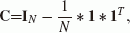 (12)
(12)where (I N ) is the N dimensional unit matrix.
-
2)
Compute the A matrix
 (13)
(13) -
3)
Employing singular value decomposition (SVD) of A, we obtain the matrices U, V and diag(λ1, λ2, λ3), where
 (14)
(14) -
4)
The rotation matrix can then be computed as (15)
 (15)
(15) -
5)
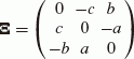
The rotation matrix in general is given by using 3 axial rotation angles (α, β, γ), but can also be expressed by the skew matrix as
 (16)
(16)Consequently, the skew matrix is
 (17)
(17)and then the parameters a, b and c can be computed from
 (18)
(18) -
6)
The scale parameter can then be expressed as
 (19)
(19)where {tr} is the trace of a matrix.
-
7)
Since the translation vector satisfies the following normal equation
 (20)
(20)we therefore obtain
 (21)
(21)For the purpose of this study, the algorithm has been implemented in Mathematica.


4. The 3D Affine Transformation Problem
The 3D affine transformation is one possible generalization of the C7(3, 3) Helmert transformation, using three different scale (s1, s2, s3) parameters instead of a single one. In this case, the scale factors can be modeled by a diagonal matrix (S).

where

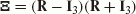
is the scale matrix, X0, Y0, Z0 are the 3 translation parameters and R is the rotation matrix. The rotation matrix can be expressed by the skew-symmetric matrix (Ξ) as in (18) which together with (16) leads to:

for which the restriction satisfy

5. ABC Procrustean Algorithm
In order to solve the 3D affine transformation problem outlined in (22), the ABC (Awange, Bae and Claessens) algorithm is implemented as follows (Awange et al., 2008):
-
1)
Compute the center of gravity of the two systems
 (26)
(26) (27)
(27) -
2)
Translate the systems into the center of the coordinate system
 (28)
(28) (29)
(29) -
3)
Compute the matrix A
 (30)
(30) -
4)
Compute the rotation matrix R via (15)
-
5)
The first approximation of the scale matrix (S0) only considers the diagonal elements of,
 (31)
(31)i.e.,
 (32)
(32) -
6)
Iterate to improve the scale matrix
 (33)
(33) (34)
(34)then after the first iteration step
 (35)
(35) -
7)
After the iteration, the scale matrix is
 (36)
(36) -
8)
Then the translational vector
 (37)
(37)


6. Extension of the ABC Method via the PZ Algorithm
The ABC method is very fast, and the computation effort for iteration to improve the S scale matrix is negligible. The main problem with the ABC method, however, is that after shifting the two systems onto the origin of the coordinate system, the rotation matrix is computed via SVD. This means that the physical rotation, as well as the deformation (distortion) caused by the different scaling in the different directions of the 3 different principal axes, will also be involved in the computation of the rotation matrix. This can be approximately allowed only when these scale factors do not differ from each other considerably. In addition, the necessary condition for obtaining the optimal scale matrix is restricted to the diagonal matrix (e.g., Eq. (36)), where the off-diagonal elements are simply deleted in every iteration step thereby leading to solutions that do not ensure a true global minimum for the trace of the error matrix.
The PZ (Paláncz-Zaletnyik) method can cure these problems, but there is a price for it! This method starts with an initially diagonal S scale matrix, and uses the inverse of this matrix to eliminate the deformation caused by scaling. Only after the elimination of this “distortion” will SVD be applied to compute the rotation matrix itself. It goes without saying that in this way, the computation of the rotation matrix should be repeated in an iterative way in order to decrease the error. That is why this method is precise and correct for any ratio of scale parameters, but takes longer to achieve the results than in the case of the ABC method.
The algorithm can be summarized as it follows:
-
1)
Use the elements of the diagonal scale matrix S in (23). The function for computing the error for the case of a given scale matrix S is the following:
-
2)
Using Eqs. (26) and (27), compute the center of gravity of the two systems.
- 3)
-
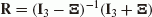
4)
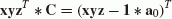
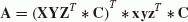
Eliminate rotation (distortion) caused by scaling with different values in different directions in the computation of matrix A using
 (38)
(38) -
5)
Compute the rotation matrix using (15).
-
6)
Compute the translation vector using (37).
-
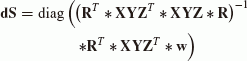
7)
Using the error matrix
 (39)
(39)compute the error matrix using (9). If this error is too high, then modify the scale matrix S, and repeat the computation. In the case of the 7-parameter similarity transformation (Helmert), the scale value (s) can be estimated by dividing the sum of length in both systems from the centre of gravity (see, Albertz and Kreiling, 1975). The center of gravity of the systems is therefore,
 (40)
(40)


The estimated scale parameter according to Albertz and Kreiling (1975) in the Helmert similarity transformation is thus given by

For the case of the 9 parameter affine transformation where 3 different scale values (s1, s2, s3) are applied to the 3 coordinate axes, a good approach for the scale parameters can be given by modifying the Albertz and Kreiling (1975) expression. Instead of the quotient of the two lengths in the centre of gravity system, we can use the quotients of the sum of the lengths in the corresponding coordinate axes directions.
The estimated scale parameters according to the modified Albertz and Kreiling (1975) expression for the 9 parameter transformation (see also Zaletnyik, 2008) is

where (s01, s02, s03) are the initial elements in (23).
Example 1: Application to a network with mild anisotropy
For the determination of the 9 transformation parameters (a, b, c, X0, Y0, Z0, s1, s2, s3), we need N ≥ 3 non-collinear points with known positions in both coordinate systems. In the case of N stations, we have 3 N nonlinear equations, a system of multivariable polynomial to solve.
First, we consider the transformation problem of the Australian Geodetic Datum (AGD 84) to Geocentric Datum Australia (GDA 94) with 82 points (e.g., Awange et al., 2008). This problem is solved using (see results in Table 1):
-
1)
Direct Numerical Solution via Global Minimization (GM). This approach solves a system of 246 equations for the unknown parameters a, b, c, s1, s2, s3, X0, Y0, Z0. In order to use directly the least squares method, we can define the objective function as the sum of the square of the errors, which should be minimized (e.g., Paláncz et al., 2008). To carry out the global minimization via a genetic algorithm, the built-in function NMinimize in Mathematica is employed. As this is the direct least squares solution of the problem, we accepted this result as reference solution.
-
2)
Application of the Helmert transformation using the original Procrustes approach.
-
3)
Application of the ABC method.
-
4)
Application of the PZ method.
The error in Table 1 and Table 2 is defined as the sum of the square of the residuals of the coordinates after the transformation.
Example 2: Application to a network with strong anisotropy
For this test, a synthetic dataset was generated from 81 Hungarian Datum points. In this case, in order to test the efficiency of the different methods, the angles of rotations are not small and the values of the 3 scale parameters are considerably different from each other. A 9-parameter transformation was applied on the original dataset, with α = 6°, β = 11.1°, γ = 16.3°, s1 = 0.62, s2 = 1.30, s3 = 1.87, and X0 = 1345.34 m, Y0 = −233.23 m, Z0 = 121.11 m. After the transformation, a normal distributed noise was added to the generated coordinate set with zero means and standard deviation of σ x = 0.07 m, σ y = 0.08 m, σ z = 0.10 m. This synthetic data was then used to estimate the original transformation parameters.
Using the four approaches defined above leads to the results of Table 2. For comparison, the second row of Table 2 contains the original data used for creating the synthetic dataset. Comparing the results, it can be seen that the Procrustes solution of the 7-parameter transformation, and the ABC method differ totally from the correct ones, whereas the PZ method has a good solution according to the residual error, since it returned the same scale parameters as the original ones, although both the translation and rotation parameters differ somewhat. The best results are achieved with the global minimization, but this calculation took the longest time. In this case, both the scale and rotation parameters are equal to the original values, but the translation parameters differ. This is because of the added normal distributed noise. The translation parameters are almost the same in case of PZ method and global minimization, and the residual error has the same magnitude. The most sensitive parameter according to the chosen method are the rotation parameters.
Example 3: Testing different initial values for the PZ algorithm
In this example, we are interested in testing the PZ-algorithm with different starting values. We consider four scenarios: (i) using an identity matrix I3 as the starting values in which case (s01 = 1, s02 = 1, s03 = 1); (ii) the modified Albertz-Kreiling expression (see Eq. (42)); (iii) the ABC-method without iteration (i.e., the results of the first run); and (iv) The ABC-method with the solutions after iterations. The results are presented in Table 3. The different initial values give the same solutions, but with different processing times, the ABC method without iteration provided the best initial value for S.
7. Conclusions
For the case of mild anisotropy in the network, the ABC method using 3D affine transformation gives a better approximation than the general Procrustes method employing Helmert transformation model, while, the PZ method provides a precise, geometrically correct solution. The ABC method is about 2 times faster than the PZ method, and the later is roughly 5 times faster than the global optimization method when applied to the 3D affine model (see Table 1).
For the case of strong anisotropy, use of the ABC method to solve the 3D affine transformation completely fails, as does the general Procrustes method for Helmert tarnsformation. The PZ method provides a good solution, and it is about 5 times faster than the global minimization. However, even in the case of strong anisotropy, the ABC method is useful for computing proper initial values for the PZ method in order to increase its efficiency (see Table 3). The different initial values give the same solutions, but with different processing times. The fastest version was that using the results of the first run of the ABC method as the initial values.
In the case of strong anisotropy, a synthetic dataset was used with known transformation parameters with added normally distributed noise. The results show that the scale factors are quite robust and insensitive to the added noise, with both the PZ method and global minimization giving back exactly the original values of the scale. The calculated translation parameters were more sensitive to the noise and differ from the original values in both cases (with 0.5%, 0.3% and 20.4%). The rotation angles were the same for global minimization, but slightly greater differences are noted with the PZ method. However, this method had the same error magnitude as the global minimization. The PZ method can be extended for a 12 parameter model, as well as for the general affine model.
The results of the computations have also been verified with the original MATLAB code of the ABC method.
References
Albertz, J. and W. Kreiling, Photogrammetric Guide, pp. 58–60, Herbert Wichmann Verlag, Karlsruhe, 1975.
Awange, J. L. and E. W. Grafarend, Solving Algebraic Computational Problems in Geodesy and Geoinformatics, Springer, 2005.
Awange, J. L., K.-H. Bae, and S. Claessens, Procrustean solution of the 9-parameter transformation problem, Earth Planets Space, 60, 529–537, 2008.
Borg, I. and P. Groenen, Modern Multidimensional Scaling, Springer, New York, 1997.
Cox, T. F. and M. A. Cox, Multidimensional Scaling, St. Edmundsbury Press, St. Edmunds, Suffolk, 1994.
Crosilla, F., A criterion matrix for a second order design of control networks, Bull. Geod., 57, 226–239, 1983a.
Crosilla, F., Procrustean transformation as a tool for the construction of a criterion matrix for control networks, Manuscripta Geodetica, 8, 343–370, 1983b.
Crosilla, F., Procrustes analysis and geodetic sciences, in Geodesy—The Challenge of the 3rd Millennium, edited by Grafarend, E. W., F. W. Krumm, and V. S. Schwarze, pp. 287–292, Springer, Heidelberg, 20
Crosilla, F. and A. Beinat, Use of generalised Procrustes analysis for the photogrammetric block adjustement by independent models, J. Photogramm. Remote Sens., 56, 195–209, 2002.
Gower, J. C., Multivariate Analysis. Ordination, Multidimensional Scaling and Allied Topics, Handbook of Applicable Mathematics, VI.: Statistics (B), 1984.
Gower, J. C. and G. B. Dijksterhuis, Procrustes Problems, New York, Oxford University Press, 2004.
Meridith, W., On weighted Procrustes and Hyperplane fitting in factor analytic rotation, Psyhometrika, 42, 491–522, 1977.
Paláncz, B., R. Lewis, P. Zaletnyik, and J. Awange, Computational study of 3D affine coordinate transformation: Part I. 3-point problem, Math-Source /7090/ and Part II. N-point problem, MathSource/7121/.: http://library.wolfram.com/infocenter/MathSource/7090/, http://library.wolfram.com/infocenter/MathSource/7121/, 2008.
Schönemann, P. H., A generalized solution of the orthogonal procrustes problem, Psychometrika, 31 (1), 1–10, 1966.
Zaletnyik, P., Coordinate transformation using Computer Algebra Systems (CAS) and Artificial Neural Netwotks (ANN), Ph.D. Dissertation, Budapest University of Technology and Economy, http://www.agt.bme.hu/staff_h/zaletnyik_pub.html, 2008.
Acknowledgements
The authors thank Dr. Kevin Fleming for proof reading the manuscript, but take the responsibility of any errors. JLA acknowledges the financial support of Alexander von Humboldt (Ludwig Leichhardt’s Memorial Fellowship) and Curtin Research Fellowship. He is grateful for the warm welcome and the conducive working atmosphere provided by his host Prof. Bernhard Heck at the Geodetic Institute, Karlsruhe Institute of Technology (KIT). TIGer Publication No. 253.
Author information
Authors and Affiliations
Corresponding author
Rights and permissions
Open Access This article is licensed under a Creative Commons Attribution 4.0 International License, which permits use, sharing, adaptation, distribution and reproduction in any medium or format, as long as you give appropriate credit to the original author(s) and the source, provide a link to the Creative Commons licence, and indicate if changes were made.
The images or other third party material in this article are included in the article’s Creative Commons licence, unless indicated otherwise in a credit line to the material. If material is not included in the article’s Creative Commons licence and your intended use is not permitted by statutory regulation or exceeds the permitted use, you will need to obtain permission directly from the copyright holder.
To view a copy of this licence, visit https://creativecommons.org/licenses/by/4.0/.
About this article
Cite this article
Paláncz, B., Zaletnyik, P., Awange, J.L. et al. Extension of the ABC-Procrustes algorithm for 3D affine coordinate transformation. Earth Planet Sp 62, 857–862 (2010). https://doi.org/10.5047/eps.2010.10.004
Received:
Revised:
Accepted:
Published:
Issue Date:
DOI: https://doi.org/10.5047/eps.2010.10.004