- Full paper
- Open access
- Published:
Bootstrapping Swarm and observatory data to generate candidates for the DGRF and IGRF-13
Earth, Planets and Space volume 72, Article number: 152 (2020)
Abstract
As posted by the Working Group V of the International Association of Geomagnetism and Aeronomy (IAGA), the 13th generation of the International Geomagnetic Reference Field (IGRF) has been released at the end of 2019. Following IAGA recommendations, in this work we present a candidate model for the IGRF-13, for which we have used the available Swarm satellite and geomagnetic observatory ground data for the last year. In order to provide the IGRF-13 candidate, we have extrapolated the Gauss coefficients of the main field and its secular variation to January 1st, 2020. In addition, we have generated a Definitive Geomagnetic Reference Field model for 2015.0 using the same modelling approach, but focussed on a 1-year time window of data centred on 2015.0. To jointly model both satellite and ground data, we have followed the classical protocols and data filters applied in geomagnetic field modelling. Novelty arrives from the application of bootstrap analysis to solve issues related to the inhomogeneity of the spatial and temporal data distributions. This new approach allows the estimation of not only the Gauss coefficients, but also their uncertainties.

Background
The study of the Earth’s magnetic field is a hot topic in Earth Sciences, since it acts as a shield protecting our planet against the solar wind and other interplanetary interactions, of major importance in our technological era. The abrupt decay of the geomagnetic dipole field, accentuated during the last century, along with the increase of the extent of the South Atlantic Anomaly, where the geomagnetic field strength presents lower values than expected for those latitudes, are some indicators for a future challenge in our scientific community (Buffett and Davis 2018; Brown et al. 2018). To properly describe the spatial and temporal evolution of the geomagnetic field, different physico-mathematical approaches can be developed using geomagnetic ground and satellite measurements. These models allow us to separate the geomagnetic field into its different sources, such as the main field generated in the Earth’s outer core, the crustal field acquired by ferromagnetic minerals during the geological processes of the lithosphere and magnetization induced in the crustal rocks by the main field, or the external field due to the Sun’s activity influence in the ionosphere and the magnetosphere.
Since the early 1970s the International Association of Geomagnetism and Aeronomy (IAGA) has provided reference models of the geomagnetic main field every 5 years, the first model being published in 1971 (Zmuda 1971): the 1st generation of IGRF (IGRF-1, International Reference Geomagnetic Field). During 2018, the IAGA launched a new call for the submission of IGRF candidates for the last generation. At the end of 2019, the 13th generation IGRF was released (https://www.ngdc.noaa.gov/IAGA/vmod/igrf.html, Alken et al. 2020). The IGRF-13 product includes the geomagnetic main field for 2020.0 and its temporal variation to extrapolate it from 2020.0 to 2025.0. In addition, it involves the revision of the previous IGRF-12 (Thébault et al. 2015a), deriving the definitive geomagnetic reference field (DGRF) for 2015.0.
With the advent of the satellite era, the IGRF products are being developed using both observatory and satellite data. Today, we are in the best condition thanks to the three identical Swarm satellites of the European Space Agency (Olsen and Haagmans 2006), which have been monitoring the geomagnetic field since November 2013 with an unprecedented sampling rate and accuracy. In addition, the geomagnetic observatory data (most of them belonging to the INTERMAGNET network) are used to better constrain the secular variation at ground level.
Taking advantage of the availability of both Swarm and observatory data, in this work we propose the three candidates for the 13th generation IGRF. Our first candidate corresponded to a DGRF model for 2015.0. The second and third candidates were an IGRF model for 2020.0 and a secular variation model to predict the geomagnetic field variations from 2020 to 2025, respectively.
Methods
Satellite data selection
We have used all the Swarm satellite data available for the considered time periods. These data correspond to the Level-1b product Mag-L (level version _0505_, i.e., the last version allocated at the ESA server in September 2019). From each Swarm satellite, the Absolute Scalar Magnetometer (ASM) has provided the scalar data denoted by F, while the Vector Field Magnetometer (VFM) has been used to get the vector data (i.e., the North X, East Y, and vertical Z components that corresponds to − Bθ, Bλ, and − Br elements in the NEC frame, respectively). In addition, ESA provides two sampling frequencies for magnetic data: 1 Hz (low resolution, denoted as LR in the files) and 50 Hz (high resolution, HR). In our study, we have used the low resolution (LR) data: one datum per second.
To get our DGRF and IGRF candidates, two different time windows were established:
-
a.
The DGRF candidate has been derived from a time-continuous parent model using Swarm data from 1st July 2014 to 30th June 2015 (1-year time window centred at 2015.0). Note that since 5th November 2014, Swarm C does not provide ASM scalar data. For this reason, we have used the ASM scalar data up to this date, after that we have estimated the scalar Swarm C element using the vector data. Daily magnetic data from Swarm A and C cover the whole time interval (365 data files for Swarm A and C). However, no data are available for Swarm B on 11th January 2015 (364 data files for Swarm B).
-
b.
The IGRF candidate was estimated from a time-continuous parent model using Swarm data from 1st September 2018 to 15th September 2019 (380 days centred at 2019.16). For Swarm A there are no data available for the days 10th and 11th June 2019 (378 data files). For Swarm B, the 17th August 2019 is not available (379 data files). For Swarm C the days 29th and 30th April 2019, 1st May 2019, and 16th July 2019 are not available (376 data files).
All the Swarm data have been selected to avoid measurements during high external geomagnetic activity. For both time windows detailed above, we have used the next selection criteria:
-
Data from dark regions, i.e., the Sun at least 10° below the horizon (satellite’s altitude).
-
VectorVFM data in non-polar regions where |QDL| ≤ 55° (QDL: quasi-dipole latitude, for whose estimation we have used the IGRF-12).
-
ScalarASM data in polar regions where |QDL| > 55°.
-
|Dst| < 30 nT for all data.
-
|ΔDst/Δt| < 2 nT/h for non-polar data, |ΔDst/Δt| < 5 nT/h for polar data.
-
ap < 10, ap (3-h before) < 12, ap (3-h after) < 12 for all data.
-
|IMF By| < 8 nT (IMF: Interplanetary Magnetic Field).
-
− 2 < IMF Bz < 6 nT.
-
Em < 0.8 mV/m for polar data (Em: merging electric field at the magnetopause. We have used the expression given for the CHAOS-6 model, Finlay et al. 2015).
-
|ScalarASM − ScalarVFM| < 3 nT.
-
|VectorVFM − VectorCHAOS-6| < 500 nT (until to April 2019, since CHAOS-6 was not available after this time). This filter was applied to each separate geomagnetic vector component.
-
|ScalarASM − ScalarCHAOS-6| < 100nT (until to April 2019, since CHAOS-6 was not available after this time).
To get the above indicated geomagnetic indices and near-Earth solar wind magnetic field and plasma parameters (1-h mean values, expect for the ap index which is provided every 3 h), we have used the OMNIWeb site of NASA (https://omniweb.gsfc.nasa.gov/form/dx1.html). Note that in the middle of September 2019 (when the candidate models were generated) there were no Dst and ap indices available in the OMNIWeb site for the period from 8th August 2019 to 15th September 2019, so we have resorted to the provisional Dst and ap indices from the World Data Center for Geomagnetism, Kyoto (http://wdc.kugi.kyoto-u.ac.jp/kp/index.html). In addition, the IMF and Em thresholds have not been used for this time interval.
After applying the selection criteria, we were left with 3,605,739 Swarm A (2,260,317 vector and 1,345,422 scalar), 3,650,850 Swarm B (2,214,244 vector and 1,436,606 scalar) and 3,549,601 Swarm C (2,229,656 vector and 1,319,945 scalar) data for the time interval established for the DGRF parent model, i.e., 1st July 2014–30th June 2015. Figure 1a, b shows the spatial and temporal distribution of Swarm A data (for the time-axis, we have used the modified Julian days relative to 2015.0). For Swarm B and Swarm C, both spatial and temporal distributions were similar. In Fig. 1, red colour represents the vector data and blue the scalar data. Swarm A presents different temporal gaps of 5-day bins as shown in Fig. 1a, b. Some of these gaps were covered by the data coming from Swarm B and Swarm C, but there was a gap of 5 days (between the modified Julian day interval 76–81 relative to 2015.0) where no Swarm data were available (this issue will be analysed in “Modelling approach” section). Another observed pattern in Fig. 1b is the larger number of Swarm A data during the summer months in the North Hemisphere (winter in the South Hemisphere, identified in the x-axis of Fig. 1b by absolute modified Julian days relative to 2015.0 higher than 90 days). This is due to the selection of data in dark regions (Sun at least 10° below the horizon) and consequently, the South Hemisphere is characterized by a larger number of Swarm A data. This pattern is corroborated by Fig. 1c, where a decreasing number of Swarm A data can be seen for increasing quasi-dipole latitudes. This behaviour was also found for the Swarm B and Swarm C data.

a, d Spatial distributions of Swarm A data according to the quasi-dipole latitude and time in modified Julian days. b, e Temporal histograms of the number of data (scalar and vector) using bins 5 days wide. c, f Number of Swarm A data as a function of the quasi-dipole latitude (bins every 2°). Upper panel: Swarm A data for DGRF parent model and modified Julian days relative to 2015.0. Lower panel: Swarm A data for IGRF parent model and modified Julian days relative to 2019.16
The IGRF parent model has been developed with 5,875,141 Swarm A (3,657,693 vector and 2,217,448 scalar), 5,806,766 Swarm B (3,608,339 vector and 2,198,427 scalar) and 5,957,684 Swarm C (3,723,674 vector and 2,234,010 scalar) data for the total time interval. As for the previous time window, we have plotted the spatial and temporal distribution of Swarm A data in Fig. 1d–f (for the time-axis, the modified Julian days are relative to 1st March 2019, approx. 2019.16). For Swarm B and Swarm C, both spatial and temporal distributions were similar. For this time interval, although Swarm A data show some 5-day bins without data (Fig. 1d, e), no gaps of 5-day bins were found for the IGRF time period considering the rest of Swarm satellite data. As seen for the DGRF time window, Fig. 1e indicates larger number of Swarm data during the South Hemisphere winter showing the decreasing pattern for increasing quasi-dipole latitudes in Fig. 1f.
Geomagnetic observatory data selection
For the DGRF parent model, we have used hourly mean vector data from a total of 159 geomagnetic observatories spanning the annual period 1st July 2014–30th June 2015. The data sets were obtained from the portal of the WDC for Geomagnetism in Edinburgh (www.wdc.bgs.ac.uk/dataportal/) and include definitive data only. A list with all the observatories (IAGA code) used for the DGRF parent model is given in Additional file 1: Table S1. For the IGRF parent model, the available 1-min vector data from a total of 75 geomagnetic observatories spanning the annual period 1st September 2018–31st August 2019 have been used. The data set was obtained from the INTERMAGNET portal (http://www.intermagnet.org/data-donnee/download-eng.php) and included the best available data type, either definitive or quasi-definitive (provisional and variation data have been excluded). Hourly mean data have been used throughout as a basis for our analysis concerning observatory data. These have been calculated from the 1-min data in this case. In Additional file 1: Table S1, we have listed all the observatories (IAGA code) used for the IGRF parent model.
A revision of the observatory data was performed based on different criteria. Since definitive or quasi-definitive observatory data were used, the scalar element has to be (nearly) consistent with the geometric sum of the vector components. Datasets not fulfilling this criterion were rejected. In addition, data were individually plotted to detect jumps in the baselines, as well as trends and spikes. In order to make this criterion more reliable, we used the prediction provided by the CHAOS-6 to assess the observations. After this revision, we have applied the following criteria for the selection of quiet-time intervals for both DGRF and IGRF parent models:
-
Local midnight hourly values: 01–02 local time.
-
Kp ≤ 1+ (ap ≤ 5) for observatories in non-polar regions.
-
AE ≤ 50 nT for observatories in polar regions for the DGRF parent model.
-
Kp ≤ 0+ (ap ≤ 2) for observatories in polar regions for the IGRF parent model (AE indices are not available for this time period).
A total of 19,167 and 10,399 vector data satisfied the above criteria selection for each DGRF and IGRF time window, respectively. It is worth noting that no baselines or crustal biases were estimated for the observatory data, since we have used the difference between two time-consecutive data (more details can be found in “Modelling approach” section). Locations of both observatory datasets are plotted in Fig. 2. The spatial distribution of the observatories (Fig. 2a, d) shows a higher concentration of them in the North Hemisphere, particularly in Europe. We have taken into account this biased distribution weighting the observatory data (see next section). In terms of time, Fig. 2b, e show good time covertures of number of data per month. Finally, the number of data provided by each observatory was represented in Fig. 2c, f, with a median of 136 and 130 observatory data per observatory for the DGRF and IGRF parent model, respectively (in Additional file 1: Table S1, we have linked the number of observatory of x-axis in Fig. 2c, f with the IAGA code).

a, d Spatial distributions of the observatories. b, e Number of observatory data per month (see time windows in the main text). c, f Number of data per observatory (x-axis numbers correspond to the IAGA code given in Additional file 1: Table S1). Upper panel: observatories for DGRF parent model. Lower panel: observatories for IGRF parent model
Weighting scheme
Satellite and observatory data have been weighted according to their spatial distribution. For observatory data, this weighting scheme is important to avoid possible biases due to the high concentration of observatories in some regions (e.g. Europe). We have used a Gaussian Kernel density function \(K\) based on the angular distance \(\alpha_{j}\) between the location (i.e., latitude and longitude) of the jth observatory and an arbitrary location:
where \(\alpha_{ji}\) is the angular distance between observatories \(j\) and \(i\) (\(i\) = 1, … \(N\)), \(N\) is the total number of observatories (i.e., \(N\) = 159 for DGRF observatories and 75 for IGRF observatories) and \(h\) is the bin size for the angular distance \(\alpha_{j}\), which ranges between 0º and 180º (\(h\) was fixed as 5° throughout).
To estimate the weight for the jth observatory, we have first calculated the corresponding mean value of \(\alpha_{j}\), which we denote \(<\alpha_{j}>\), using the density function \(K\left( {\alpha_{j} } \right)\) (Eq. 1). Note that, \(<\alpha_{j}>\) can be understood as the mean angular distance between observatory \(j\) and the whole dataset. Secondly, all the \(<\alpha_{j}>\) mean values (\(j\) = 1, … \(N\)) were normalized by the minimum mean angular distance \(\alpha_{ \hbox{min} }\) obtained from all the observatories (this value was found to be 50º for both DGRF and IGRF datasets), providing weights wj = \(<{{\alpha_{j} } >\mathord{\left/ {\vphantom {{\alpha_{j} } {\alpha_{ \hbox{min} } }}} \right. \kern-0pt} {\alpha_{ \hbox{min} } }}\) between 1.0 and 2.4 (these weights were included in Additional file 1: Table S1). As expected, observatory data from Europe had weights close to 1, whereas the isolated observatories, such as those located in the Pacific or Antarctic regions, had the largest weights (up to 2.4).
For Swarm data, we have used the same approach. In this case, our modelling technique (see “Modelling approach” section) imposes a homogeneous spatial distribution for the satellite data. Consequently, all Swarm data had the same weight fixed as 1.8 (corresponding to a mean angular distance of 90º calculated from Eq. 1).
In terms of time, no weighting scheme has been applied. However, for the observatory data, we have selected the data following a homogenous distribution in time with a fixed number of data per month (see “Modelling approach” section). In addition, we have used two different quality observatory data: definitive data for the DGRF, and quasi-definitive (or definitive when available) data for the IGRF. However, no weighting scheme was applied in terms of this quality of data.
Modelling approach
Below, we have listed the steps to jointly model both vector and scalar data (the same procedure has been used for DGRF and IGRF parent models):
-
Step 1. Satellite input data.
A grid of 1000 nodes homogeneously distributed over the sphere was used to resample the Swarm data. Each node in this grid represents a spherical cap of approximately 3.3° semi-angle over the sphere (see Fig. 3). We have used 3 different grids for Swarm A, B, C satellites obtained from the same 1000-node grid, but slightly rotated over the sphere for each Swarm satellite. The 1000 spherical caps were used to distribute the Swarm data in areas homogeneously distributed over the sphere. Figure 3 shows an example of the spatial distribution, in terms of spherical caps of 3.3°, for the Swarm A data for the time window of the DGRF parent model. We have divided the vector and scalar data in two geographic maps according the quasi-dipole latitude using ± 55º as a threshold, where the spherical caps were coloured following the colour-bar of the number of Swarm A data within each spherical cap.
Fig. 3 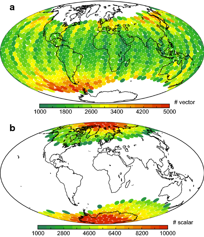
a Total number of vector Swarm A data within the spherical caps of 3.3° semi-angle for the period 1st July 2014 to 30th June 2015. b Same for the scalar Swarm data
In Additional file 2: Figure S1 we have provided histograms of the number of Swarm data within each spherical cap for the three Swarm satellites and for both DGRF and IGRF parent models. For the DGRF time window, all the spherical caps contained more than 2000 data (approx. median of 2800 data per spherical cap). Only 46/68/52 spherical caps from Swarm A/B/C, respectively, had a number of data lower than 2000. In none spherical cap there was less than 1500 data. For the IGRF time window, we had more data per spherical cap: median of approx. 4500 data per spherical cap. Only 39/61/20 spherical caps from Swarm A/B/C, respectively, had a number of data lower than 3500. In none spherical cap there was less than 2900 data. We had more data for the IGRF parent model than for the DGRF because of: (i) the IGRF time window is characterized by lower external geomagnetic activity than the DGRF time window, (ii) the IGRF time window has 15 days more than the DGRF, and (iii) some filters were not applied to reject data in the IGRF time window from 8th August 2019 to 15th September 2019.
After distributing the Swarm data within the spherical caps, we have selected a sub-dataset of Swarm data. To do that, a fixed number of Swarm data for each spherical cap was randomly picked: 4 data for Swarm A and Swarm C that both fly approximately at the same altitude of ca. 465 km (i.e., 2 data for Swarm A and 2 for Swarm C) and 4 data for Swarm B that flies ca. 520 km altitude. Consequently, the random sub-dataset contained 2000 Swarm A data, 4000 Swarm B data and 2000 Swarm C data (in total, 8000 data). We have chosen these numbers of Swarm data after carrying out several case studies using synthetic data from the CHAOS-6 model estimated in the same geocentric coordinates and dates than the complete Swarm databases. This procedure was repeated 1000 times obtaining 1000 different random datasets of 8000 Swarm data each. Note that for each dataset, the 8000 Swarm random data are homogeneously distributed over the sphere.
-
Step 2. Observatory input data.
We have randomly resampled the observatory data, keeping N data per month for each observatory (when available) with N = 2 and 4 for the DGRF and IGRF parent models, respectively. Each time window contains 12 months, and consequently, we had 12 × N × D observatory data per year, where D is the number of observatories used (D = 159 for the DGRF parent model and D = 75 for the IGRF parent model). This procedure provided, for each parent model, a number of observatory data of ~ 4000 at ground level, similar to the Swarm data (4000 data at Swarm A/C altitude and 4000 data at Swarm B altitude). We have repeated this procedure 1000 times and again, we got 1000 different random datasets of observatory data.
-
Step 3. Model parametrization.
Using the first 8000-dataset of Swarm data and the first dataset of 12 × N × D observatory data, we have developed a first parent model for both DGRF and IGRF following a weighted least-squares inversion. For each parent model, we have estimated the core field using the classical expansion of the geomagnetic potential in spherical harmonic functions from degree n = 1 to 20 with Gauss coefficients \(g_{n}^{m}\) (and \(h_{n}^{m}\)) linearly depending on time:
$$g_{n}^{m} \left( t \right) = \left. {g_{n}^{m} } \right|_{{t_{0} }} + \left. {\dot{g}_{n}^{m} } \right|_{{t_{0} }} \cdot\left( {t - t_{0} } \right),$$(2)where \(t_{0}\) is a reference date for each parent model (\(t_{0}\) = 2015.0 for DGRF and 2019.16 for IGRF). This means an estimation of 880 parameters representing the core field: 440 parameters for the Gauss coefficients at \(t_{0}\) and 440 parameters for the secular variation. In terms of spatial resolution, it is worth noting that the selected maximum harmonic degree n = 20 provided a minimum spatial wavelength of ~ 2150 km at Swarm altitude. This value is larger than the mean separation between Swarm data within two neighbour spherical caps (~ 790 km that corresponds to two spherical nodes separate around 6.6º at Swarm altitude).
To model the external field, we have followed the methodology proposed for the last CHAOS model (Finlay et al. 2015) using the external potential expression:
$$\begin{aligned} V^{\text{ext}} & = a\mathop \sum \limits_{n = 1}^{2} \mathop \sum \limits_{m = 0}^{n} \left( {\frac{r}{a}} \right)^{n} P_{n}^{m} \left( {{ \cos }\theta_{d} } \right)\left[ {q_{n}^{m} { \cos }\left( {mT_{d} } \right) + s_{n}^{m} { \sin }\left( {mT_{d} } \right)} \right] + \\ & \quad \; a\mathop \sum \limits_{n = 1}^{2} q_{\text{GSM}} ,_{n}^{0} R_{n}^{0} \left( {r,\theta_{\text{GSM}} , \lambda_{\text{GSM}} } \right). \\ \end{aligned}$$(3)The first addend represents the near magnetospheric sources using a harmonic expansion in solar magnetic coordinates (\(r, \theta_{d} , T_{d}\)). For this term, the degree-1 coefficients (\(q_{1}^{0} , q_{1}^{1} , s_{1}^{1}\)) depend on time as a function of both induced and external Dst index (or magnetospheric ring current index, RC, Olsen et al. 2014) as follows (same mathematical development can be derived for \(s_{1}^{1}\)):
$$q_{1}^{m} \left( t \right) = \hat{q}_{1}^{m} \left[ {E\left( t \right) + I\left( t \right)\left( {\frac{a}{r}} \right)^{3} } \right] + \Delta q_{1}^{m} \left( t \right),$$(4)where \(E\left( t \right)\) and \(I\left( t \right)\) represent the external and induced Dst or RC indices, respectively. \(\hat{q}_{1}^{m}\) is a constant parameter to be determined and \(\Delta q_{1}^{m} \left( t \right)\) represent a set of temporal baseline corrections homogeneously distributed within the considered time window. Following Finlay et al. (2015), we have estimated \(\Delta q_{1}^{0} \left( t \right)\) in bins of 5 days and \(\Delta q_{1}^{1} \left( t \right)\) and \(\Delta s_{1}^{1} \left( t \right)\) in bins of 30 days for both DGRF and IGRF parent models. The second addend represents the remote magnetospheric currents by using a spherical harmonic expansion in terms of the geocentric solar magnetospheric (GSM) coordinates (\(r, \theta_{\text{GSM}} , \lambda_{\text{GSM}}\)). No induced terms were considered here and then \(R_{n}^{0} \left( {r,\theta_{\text{GSM}} ,\lambda_{\text{GSM}} } \right) = \left( {\frac{r}{a}} \right)^{n} P_{n}^{0} \left( {\cos \theta_{\text{GSM}} } \right).\)
According to this potential expansion, the external field was estimated by 10 constant parameters (3 \(\hat{q}_{1}^{m} , 5\: \hat{q}_{2}^{m}\), and 2 \(q_{GSM} ,_{n}^{0}\)) plus 99 baselines (73 for \(\Delta q_{1}^{0} ,\) 13 \(\Delta q_{1}^{1}\), 13 \(\Delta s_{1}^{1}\)) for the DGRF parent model and 102 baselines (76 for \(\Delta q_{1}^{0} ,\) 13 \(\Delta q_{1}^{1}\), 13 \(\Delta s_{1}^{1}\)) for the IGRF parent model.
In summary, for the DGRF parent model we have simultaneously estimated a total of 989 parameters (880 for the core field and 109 for the external field), while for the IGRF parent model, 992 parameters (880 for the core field and 112 for the external field) were calculated.
In order to jointly model both vector (non-polar areas) and scalar (polar areas) data, we have applied a linearization approach for the scalar element that depends on the matrix of spatial and temporal parameters of both internal and external spherical harmonic expansions. This linearization involves the use of an iterative approach using an initial model, for which we have used a constant axial dipole field of -30,000 nT as the \(g_{1}^{0}\) Gauss coefficient (a null starting external field was considered). The inversion problem was carried out using the iterative least-squares method using the weight matrix \(W\) described in “Weighting scheme” section:
$$m_{i + 1} = m_{i} + \left( {A_{i}^{'} \cdot W \cdot A_{i} } \right)^{ - 1} A_{i}^{'} \cdot W \cdot \left( {A_{i} \cdot m_{i} - \delta } \right),$$(5)where \(m_{i}\) is the vector containing both core and external coefficients and baselines for the iteration \(i\). \(A_{i}\) is the matrix of parameters calculated by using the Fréchet derivative around the iteration \(i\), and \(\delta\) is the vector with the input data.
Finally, it is worth mentioning other considerations applied in our modelling approach:
-
a.
The observatory data constrain the secular variation, since we have used the differences between two time-consecutive data.
-
b.
To estimate the external field, we have used both satellite and observatory data. For the DGRF parent model we have used the RC index of Finlay et al. (2015) (http://www.spacecenter.dk/files/magnetic-models/CHAOS-6/), while the Dst index obtained from the NOAA database (https://www.ngdc.noaa.gov/geomag/est_ist.shtml) has been used for the IGRF parent model.
-
c.
The crustal field has been pre-estimated and removed from the satellite data using the crustal model LCS-1 (http://www.spacecenter.dk/files/magnetic-models/LCS-1/, Olsen et al. 2014). No crustal field is extracted from the observatory data, since we have used consecutive time differences and, consequently, it is automatically removed.
-
d.
No type of regularization at the core–mantle boundary (CMB) has been applied in our modelling inversion.
The parent models converged after 4 iterations. Figure 4 shows an example of the relative differences for the estimated parameters contained in the vector \(m\) between consecutive iterations, i.e., \(\left( {m_{i + 1} - m_{i} } \right)/m_{i}\), for the first input dataset of the DGRF parent model. Before the first iteration all parameters of \(m_{0}\) were zero (except \(g_{1}^{0}\) = − 30,000 nT) and then we plotted the results after the second iteration. The iteration 2, represented by \({{\left( {m_{2} - m_{1} } \right)} \mathord{\left/ {\vphantom {{\left( {m_{2} - m_{1} } \right)} {m_{1} }}} \right. \kern-0pt} {m_{1} }}\), shows the large magnitude differences for the lowest harmonic degrees of the internal field. Then consecutive iterations represent small convergences to the final values. As shown in Fig. 4, after 4 iterations, no differences are practically observed.
Fig. 4 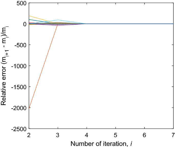
Relative difference between consecutive model coefficients as a function of the number of iterations for one of the 1000 ensembles for the DGRF parent model
-
a.
-
Step 4. Bootstrap to generate robust ensembles of 1000 parent models.
We have repeated the previous steps (1 to 3), but now using the second dataset of 8000 Swarm data and the second dataset of 12 × N × D observatory data, obtaining a new set of coefficients and baselines for the parent models. Successively and using the 1000 sub-datasets, we obtained an ensemble of 1000 parent models. The ensemble of parent models provided 1000 sets of Gauss coefficients (and baselines) that follow pretty well a Gaussian or normal distribution. Figure 5 shows the histograms of some Gauss coefficients (and baselines) for the ensemble of 1000 parent models for the DGRF and IGRF. To clearly see the fitting to a normal distribution, the theoretical Gaussian curves with same mean and standard deviation were also plotted in red lines.
Fig. 5 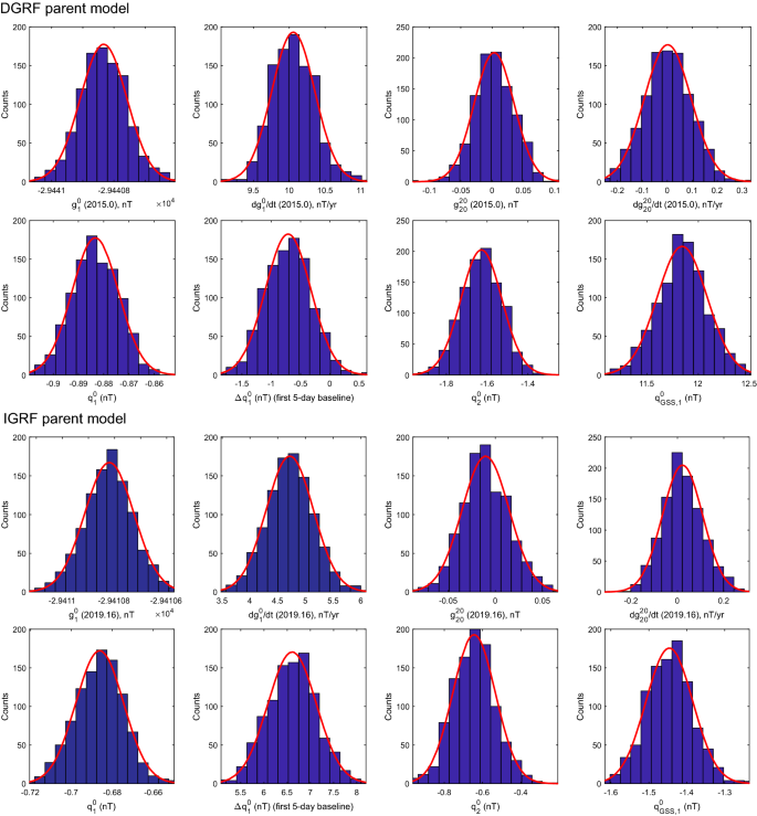
Some Gauss coefficients and baseline corrections for both (upper panel) DGRF and (lower panel) IGRF parent models. Red lines show theoretical Gaussian distribution calculated from the mean and the standard deviation of the dataset
Using this normal distribution, we have estimated the mean value and the 1-σ uncertainty for each coefficient (or baseline) distribution, which depends on the spatial and temporal input data distribution. This approach provides robust outputs (ensemble models) to better estimate the mean Gauss coefficients. However, in order to better estimate the Gauss coefficient uncertainties a realistic data covariance matrix should be used during the inversion approach. This was not performed in our study and therefore the model uncertainties could present some limitations.
Another important point of the bootstrap approach is to analyse how each coefficient was constrained in time. The modelling approach involved a linear time behaviour to all the internal Gauss coefficients (see Eq. 2), so a few number of data per temporal bins was enough to get robust linear fittings. This was not the case of the external Gauss coefficients, where the number of data per temporal bins played an important role. To deeply analyse this issue, we have plotted histograms (see Additional file 3: Figure S2) with bins of 5 days and 30 days using the 1000 datasets of Swarm data for both DGRF and IGRF parent models (same temporal bins used to constrain the external field). Each histogram shows the mean number of data and its standard deviation, both obtained from the 1000 datasets. The histograms of 5-day bins (Additional file 3: Figure S2a, c) allowed us to know how the baselines of the external Gauss coefficient \(q_{1}^{0}\) were constrained during the inversion process. All the bins presented a number of data higher than 12 (for DGRF) and 20 (for IGRF), an enough number of data to estimate a constant baseline \(\Delta q_{1}^{0}\) per bin. As indicated in “Satellite data selection” section, there was one bin in Additional file 3: Figure S2a without data (modified Julian day interval 76–81 relative to 2015.0). Consequently, this baseline was not estimated for the DGRF parent model, but it did not affect to the final DGRF candidate. Logically, the histograms of 30-day bins (Additional file 3: Figure S2b, d) show a more homogenous time distribution. This number of data per bin was enough to estimate the baselines for the external Gauss coefficients \(q_{1}^{1}\) and \(s_{1}^{1}\) during the inversion approach.


Results and discussion
DGRF candidate
The obtained set of average Gauss coefficients and baselines for the DGRF parent model allowed calculating data residuals and the root mean square (RMS) error for the Swarm and observatory data.
Concerning the Swarm data, the residuals were calculated for each Swarm satellite. Results for the Swarm A are plotted in Fig. 6 (for Swarm B and C, see Additional files 4, 5: Figures S3 and S4, respectively). Table 1 contains the mean and RMS errors for each Swarm satellite and the whole Swarm dataset. For each geomagnetic element, we have calculated and represented the spatial RMS error within each spherical cap, as detailed in the previous section of Swarm data selection. RMS error maps (column a in Fig. 6, Additional files 4, 5: Figures S3 and S4) show similar patterns for the three Swarm satellites, with higher values toward polar areas (in particular for the scalar F maps, where data cover all latitudes). For the vector data, no RMS errors were calculated and plotted for the spherical caps within polar regions. The vertical component (Z) shows the lowest RMS values, with an average error of 3.14 nT for Swarm A, or 3.10 nT if we account for all Swarm data (see Table 1).

RMS errors for each vector and scalar elements for the Swarm A data. Columns (a) and (c) represent the maps of the RMS errors for the DGRF and IGRF parent models, respectively. Columns b) and d) provide the RMS errors as a function of the modified Julian days relative to 2015.0 and 2019.16 for DGRF and IGRF, respectively
We have also plotted the RMS errors as a function of time (column b in Fig. 6, Additional files 4, 5: Figures S3 and S4). For each geomagnetic element, RMS errors in 5-day bins show similar values throughout the DGRF time window, with lower RMS errors observed in the Z component and the scalar F (in non-polar regions) for the three Swarm satellites. Note that we have divided the scalar F (lower histogram in column b) into polar (yellow bars) and non-polar regions (orange bars).
Concerning the geomagnetic observatory data, the residuals were calculated using the total set (see Fig. 7, Additional file 6: Figure S5, and Table 2). For each geomagnetic element, we have used the same input data as in the modelling approach, i.e., the differences (denoted as dX, dY, dZ, and dF) in two time-consecutive observatory measurements, thus avoiding the crustal anomaly biases. As in the Swarm case, the observatory RMS errors present higher values toward polar regions (see Fig. 7a), with higher RMS for the X and Z components (and consequently for the scalar F). This can be due to the effect of ionospheric Hall currents predominantly flowing in the east–west direction, thus giving rise to ground magnetic variations contained in the meridional plane at those high latitudes. For non-polar regions, the highest RMS errors are found in the horizontal components X and Y. Additional file 6: Figure S5 contains the observatory RMS errors versus time for each geomagnetic component, but using only the data in non-polar regions. These RMS errors show higher values during the 100 days before 2015.0.

RMS errors for each vector and scalar elements for the observatory data used in the a DGRF and b IGRF parent models
Finally, our DGRF candidate was obtained from the ensemble of 1000 DGRF parent models for a time t = 2015.0 and using the harmonic degrees 1 to 13 (core field). The ensemble of 1000 DGRF parent models provided not only the average value of the 195 Gauss coefficients, but also their uncertainties given by the standard deviation of each normal distribution (see Fig. 5, upper panel). Figure 8a, b shows the values of the Gauss coefficients and their uncertainties for our DGRF candidate, respectively. The numerical values of the Gauss coefficients are contained in Additional file 7: Table S2. The uncertainties of the Gauss coefficients (Fig. 8b) decrease with the order m for each harmonic degree n. We have also calculated the power spectrum PS (Lowes 1974) of the DGRF candidate at both Earth’s surface and at CMB (Fig. 8d). The log10 of the PS at the Earth’s surface shows the classical linear trend decay, while the estimated PS at the CMB shows the characteristic constant trend (around 1010 nT2) for the non-dipole harmonic degrees.

DGRF candidate model. a Gauss coefficients and b the uncertainties given by the 1-σ of their normal distributions. c Gauss coefficient differences between our DGRF candidate and the published DGRF-2015 model. d Power spectrum at the Earth’s surface (blue line referred to the left y-axis) and at the CMB (red line referred to the right y-axis). Differences of the power spectrum between our candidate and the DGRF-2015 model is also given by dashed lines (blue at Earth’s surface and red at CMB)
A comparison between our DGRF candidate and the final published version of the DGRF-2015 (Alken et al. 2020) has been carried out in terms of the differences for the Gauss coefficients (Fig. 8c). The largest differences were centred in the odd zonal Gauss coefficients \(g_{1}^{0}\), \(g_{3}^{0}\), and \(g_{5}^{0}\), with absolute differences around 0.6 nT, while the rest of the differences ranged between − 0.2 and 0.2 nT. The Gauss coefficient RMS error, calculated following the Lowes–Mauersberger geomagnetic PS (see Eq. 7 in Thébault et al. 2015b) was 3.20 nT. It is worth noting that the differences between our DGRF candidate and the DGRF-2015 (Fig. 8c) presented values one order of magnitude larger than the model candidate uncertainties (Fig. 8b). This is presumably because we have not managed the model uncertainties using an appropriate covariance matrix and therefore our uncertainties present this limitation. We have also plotted the residuals of the PS in Fig. 8d (dashed lines) which show larger values for higher harmonic degrees n, in particular for that calculated at the CMB.
Finally, we have represented the differences (between our DGRF candidate and DGRF-2015) of the geomagnetic components at the Earth’s surface in Fig. 9. Residual maps for the X and Z components (Fig. 9, column a) present large residuals in the harmonic zonal areas with maxima toward polar regions, characteristic of ionospheric and auroral signatures. It is worth noting the asymmetric dipolar pattern in the residuals of the Z component. These patterns are linked to the large difference presented just in the zonal odd coefficients \(g_{1}^{0}\), \(g_{3}^{0}\) and \(g_{5}^{0}\). However, we found large values not only in the previous zonal terms, but the tesseral coefficient differences with odd degree and order m = 1 also provided large differences with the DGRF-2015 (see Fig. 8c). This issue led us to think that the source of these large residuals can correspond to an incorrect separation between internal and external contributions, since we have not taken into account all the external terms in our DGRF parent model. To deeply analyse this issue, we followed the recommendation of a reviewer to compare the external field at 2015.0 with that given by the CHAOS-6 model. Results (see Additional file 8: Figure S6) show that although our DGRF parent model provides an external field similar to that provided by CHAOS-6 at 2015.0, there are some small differences just for the lowest harmonic degrees. This could be the responsible of the differences between our candidate and the DGRF-2015, since our internal coefficients could be contaminated by some external contributions.

Maps of vector components for the residuals obtained by the comparison of our candidates and the final IGRF-13 products. a DGRF residuals, b IGRF residuals, c secular variation residuals
IGRF candidate
As with the DGRF candidate, we have calculated the mean and RMS from the residuals between the input data and the average IGRF parent model obtained from the 1000 ensemble of models.
For the Swarm data, Fig. 6, Additional files 4, 5 Figures S3 and S4, and Table 1 show means and RMS values obtained from residuals of each geomagnetic element (the residuals of the scalar element in the non-polar regions were also estimated). Again, the strength field F in polar regions presented the highest RMS (column c in Fig. 6, Additional files 4, 5: Figures S3 and S4) in comparison with the other elements in non-polar regions. In these figures, maps of the Z component show the lowest spatial RMS errors, with average values of 3.26 and 3.13 nT for Swarm A and all Swarm data, respectively. Also note that for the scalar F, we found slightly higher RMS errors following the magnetic equator for the three Swarm satellites, a pattern that was not found for the vector components and for the DGRF parent model. The RMS errors versus time were plotted in the column d of Fig. 6, Additional files 4, 5: Figures S3 and S4. Here, it is important to note the largest RMS values at the end of the time windows (after the day 100 relative to 2019.16), where the Swarm data were not filtered by some parameters of the external field.
The comparison between the IGRF parent model and the geomagnetic observatory input data is provided in Table 2 and Fig. 7 and Additional file 6: Figure S5. As with the DGRF, we have estimated the residuals taking into account two time-consecutive measurements for each observatory dataset, denoted as dX, dY, dZ and dF. Again, RMS errors increase toward polar regions with larger RMS for the X and Z component (see Fig. 7b). In non-polar regions, lower RMS errors are characteristic of the vertical component Z. The RMS errors versus time (Additional file 6: Figure S5) show high values in the second half of the time window for the vector elements. These high RMS errors were expected, since this period was characterized by a high density of quasi-definitive observatory data (with lower quality than the definitive data).
Our IGRF and SV candidates were obtained from the 1000 ensemble of IGRF parent models from September 1st 2018 to September 15th 2019 using a linear extrapolation until 2020.0 as follows:
The core field (IGRF-13 candidate product) was derived from the average ensemble of IGRF parent models for degrees 1 to 13 using Eq. (6), while the secular variation (SV-2020-2025 candidate product) for degrees 1 to 8 was derived using Eq. (7). Figure 10 shows this extrapolation for the first Gauss coefficient (dashed lines indicate the Gauss coefficient uncertainty).

Extrapolation of the IGRF parent model to 2020.0 for \(g_{1}^{0}\)
The set of Gauss coefficients of the IGRF candidate is shown in Fig. 11a (mean values) and b (uncertainties of each normal distribution), and in Additional file 7: Table S2. As with previous DGRF candidates, the uncertainties of the Gauss coefficients decrease with the order m for each harmonic degree n. Using the mean Gauss coefficients, we have represented the PS at the Earth’s surface and at the CMB (Fig. 11d). Finally, we have also compared our IGRF candidate with the final IGRF-2020 (Alken et al. 2020). The largest difference (see Fig. 11c) between candidate and final model corresponded to the axial dipole field (coefficient \(g_{1}^{0}\)), with ca. 2 nT absolute difference, and the rest of the differences ranged between − 0.4 and 0.4 nT with an RMS error (calculated using the Lowes-Mauersberger power spectra) of 8.87 nT. The residuals of the PS are also plotted in Fig. 11d, where the highest harmonic degree n presented again the largest residuals, in particular for those estimated at the CMB.

IGRF candidate model. a Gauss coefficients and b the uncertainties given by the 1-σ of their normal distributions. c Gauss coefficient differences between our IGRF candidate and the published IGRF-2020 model. d Power spectrum at the Earth’s surface (blue line referred to the left y-axis) and at the CMB (red line referred to the right y-axis). Differences of the power spectrum between our candidate and the IGRF-2020 model is also given by dashed lines (blue at Earth’s surface and red at CMB)
Global maps of residuals (between our IGRF candidate and the IGRF-2020) for the vector geomagnetic elements are plotted in Fig. 9 (column b). We found general patterns opposite to those described for the X and Z maps of the DGRF candidate (Fig. 9, column a). The reason was that for the IGRF comparison the largest difference was given by the axial Gauss coefficient \(g_{1}^{0}\) with negative residual (− 2.07 nT), and for the DGRF comparison the largest residual was also given by \(g_{1}^{0}\) but with a positive difference value (0.63 nT), providing the opposite colour patterns in maps of X and Z of DGRF and IGRF candidates. As for the DGRF, the origin of this high residuals, apart from the difference found for the \(g_{1}^{0}\), came from other zonal coefficients (\(g_{3}^{0}\) and \(g_{5}^{0}\)) and tesseral coefficients with order m = 1 (see Fig. 11c). We have again considered that an incorrect separation between internal and external contributions was the key to these differences. In effect, as seen in the DGRF parent model, we have found some discrepancies between the external field of the IGRF parent model at 2019.16 and that provided by the CHAOS-6 for the same date (see panel b in Additional file 8: Figure S6).
Secular variation candidate
The first time derivative of the Gauss coefficients, i.e., the secular variation, from degree 1 to 8 has provided our secular variation candidate model (SV candidate) from 2020 to 2025. Figure 12 shows these coefficients (Fig. 12a) and their uncertainties (Fig. 12b) whose values are given in Additional file 7: Table S2. In Fig. 12c, we have compared our SV candidate with the final published SV-2020-2025 model (Alken et al. 2020). The RMS error (in terms of the Lowes-Mauersberger PS) of these differences was 5.64 nT/year, with the largest absolute difference (about 1 nT/year) found for the axial dipole coefficient \(g_{1}^{0}\). The secular variation of the PS was also estimated at the Earth’s surface and at the CMB (Fig. 12d). The secular variation of the PS presents a maximum for the harmonic degree n = 2 at the Earth’s surface and an increasing trend for all harmonic degrees at the CMB. Secular variation of the PS differences with the SV-2020-2025 model is larger for higher harmonic degrees.

SV candidate model. a Secular variation of the Gauss coefficients and b their uncertainties given by the 1-σ of their normal distributions. c Secular variation of the Gauss coefficient differences between our SV candidate and the published SV-2020-2025 model. d Secular variation of the power spectrum at the Earth’s surface (blue line referred to the left y-axis) and at the CMB (red line referred to the right y-axis). Differences of the secular variation of the power spectrum between our candidate and the SV-2020-2025 model is also given by dashed lines (blue at Earth’s surface and red at CMB)
Finally, in column c of Fig. 9 we have plotted the residual maps for the three vector components (differences between our SV candidate and the SV-2020-2025 model). An important residual anomaly can be found around the north magnetic pole in the three maps, which can be explained by the large negative differences found in the axial coefficients \(g_{n}^{0}\), in particular for \(n =\) 1, 2, 4 and 8. In addition, the high residuals in the Pacific region (in particular for the residual maps of X and Z components) can be explained by the large difference of the tesseral coefficients \(h_{n}^{1}\), in particular for even \(n + m\)(\(n =\) 5 and 7).
Conclusion
The team, consisting of researchers from different Spanish institutions (UCM, CSIC, OE, ROA, and IGN), has derived three candidate models for the 13th generation IGRF. To do that, we have developed two time-continuous parent models based on both main and external geomagnetic fields. From the first parent model, extended from 1st July 2014 to 30th June 2015, we have derived our 2015 DGRF candidate of the core field truncated to spherical harmonic degree 13. The second parent model, developed between September 1st 2018 and September 15th 2019, has provided both 2020 IGRF and SV-2020-2025 candidate models. These candidates were truncated to spherical harmonic degree 13 for the IGRF and degree 8 for the SV-2020-2025. Bootstrapping has allowed us to estimate a robust set of mean Gauss coefficients and their secular variation, but some limitations were found in terms of the uncertainties since we have not used a more realistic covariance matrix in the inversion approach. In addition, all the three candidates have been compared with the final published product IGRF-13 showing Lowes-Mauersberger RMS errors of 3.20 nT, 8.87 nT, and 5.64 nT/yr for the DGRF, IGRF, and SV candidates, respectively. From these comparisons with the final IGRF-13 products, we realized that our candidates shown some inconsistences for lower order harmonic coefficients (in particular for the axial \(g_{n}^{0}\) and \(g_{n}^{1}\) − \(h_{n}^{1}\) Gauss coefficients) originated by an incorrect separation between internal and external contributions during the modelling inversion. These findings will help us to improve our new bootstrap approach to provide further robust candidates for the next generation of IGRF-14 to be released in 2025.
Availability of data and materials
All datasets used in this study can be found in the respective webpages indicated along the manuscript.
Abbreviations
- CMB:
-
Core–mantle boundary
- DGRF:
-
Definitive geomagnetic reference field
- IAGA:
-
International Association of Geomagnetism and Aeronomy
- IGRF:
-
International Geomagnetic Reference Field
- SV:
-
Secular variation
References
Alken P et al (2020) International geomagnetic reference field: the thirteenth generation. Earth Planets Space. https://doi.org/10.1186/s40623-020-01288-x
Brown M, Korte M, Holme R, Wardinski I, Gunnarson S (2018) Earth’s magnetic field is probably not reversing. Proc Natl Acad Sci 115(20):5111–5116
Buffett B, Davis W (2018) A probabilistic assessment of the next geomagnetic reversal. Geophys Res Lett 45(4):1845–1850
Finlay CC, Olsen N, Tøffner-Clausen L (2015) DTU candidate field models for IGRF-12 and the CHAOS-5 geomagnetic field model. Earth Planets Space. https://doi.org/10.1186/s40623-015-0274-3
Lowes FJ (1974) Spatial power spectrum of the main geomagnetic field and extrapolation to the core. Geophys J R Astr Soc 36:717–730
Olsen N, Haagmans R (2006) Swarm-the Earth’s magnetic field and environment explorers. Earth Planets Space 58:349–496
Olsen N, Lühr H, Finlay CC, Sabaka TJ, Michaelis I, Rauberg J, Tøffner-Clausen L (2014) The CHAOS-4 geomagnetic fieldmodel. Geophys J Int 1997:815–827
Thébault E, Finlay CC, Beggan CD, Alken P, Aubert J, Barrois O, Canet E (2015a) International geomagnetic reference field: the 12th generation. Earth Planets Space 67(1):79. https://doi.org/10.1186/s40623-015-0228-9
Thébault E, Finlay CC, Alken P, Beggan CD, Canet E, Chulliat A, Rother M (2015b) Evaluation of candidate geomagnetic field models for IGRF-12. Earth Planets Space 67(1):112. https://doi.org/10.1186/s40623-015-0273-4
Zmuda AJ (1971) The International Geomagnetic Reference Field: introduction. Bull Int Assoc Geomag Aeronomy 28:148–152
Acknowledgements
The authors are grateful to the Spanish research project PGC2018-099103-A-I00 of the Spanish Ministry of Science, Innovation and Universities. We would like to thank the editors of this special issue and two anonymous reviewers for their useful comments. We are also grateful to the task force team of the Working Group V of IAGA for promoting and evaluating the IGRF-13 candidates. We also thank ESA for providing the Swarm Level-1b data. This work has used geomagnetic observatory data and we thank all the research institutions and observatories that provide these data, most of them supported by the INTERMAGNET network. Finally, a special dedication to all the people who are suffering the present pandemic situation, and in particular to all of them working for us while we rest at home.
Funding
This work has been funded by the project PGC2018-099103-A-I00 entitled “Candidato Español para Campo Geomagnético de Referencia Internacional 2020” under the umbrella of the programme “I + D de Generación de Conocimiento” of the Spanish Ministry of Science, Innovation and Universities.
Author information
Authors and Affiliations
Contributions
FJPC generated the 2015-DGRF, 2020-IGRF and SV-2015-2020 candidates. SM and JMTorta compiled, selected and analysed all the geomagnetic observatory data. FJPC, SM, JMTorta drafted the manuscript. MC, FMH and JMTordesillas contributed to improve the manuscript. All authors read and approved the final manuscript.
Corresponding author
Ethics declarations
Ethics approval and consent to participate
Not applicable.
Consent for publication
Not applicable.
Competing interests
The authors declare that they have no competing interests.
Additional information
Publisher's Note
Springer Nature remains neutral with regard to jurisdictional claims in published maps and institutional affiliations.
Supplementary information
Additional file 1: Table S1.
List of observatories used in the DGRF and IGRF parent models. First column is the associated number used in Fig. 2 of the main text, second column is the IAGA code, and third column is the spatial weight used in the modelling approach.
Additional file 2: Figure S1.
Number of Swarm data within each of the 1000 considered spherical caps for the a) Swarm A, b) Swarm B and c) Swarm C satellites for the (upper panel) DGRF and (lower panel) IGRF parent models.
Additional file 3: Figure S2.
Number of Swarm data for each sub-dataset of 8000 Swarm data (see text for details) considering temporal bins of 5 days (a and c) and 30 days (b and d). Upper panel: data for the DGRF parent model. Lower panel: data for the IGRF parent model. Each column contains the mean ± standard deviation of the number of data within the temporal bin calculated from the 1000 sub-datasets of 8000 Swarm data each.
Additional file 4: Figure S3.
RMS errors for each vector and scalar elements for the Swarm B data. Columns (a) and (c) represent the maps of the RMS errors for the DGRF and IGRF parent models, respectively. Columns (b) and (d) provide the RMS errors as a function of the modified Julian days relative to 2015.0 and 2019.16 for DGRF and IGRF, respectively.
Additional file 5: Figure S4.
RMS errors for each vector and scalar elements for the Swarm C data. Columns (a) and (c) represent the maps of the RMS errors for the DGRF and IGRF parent models, respectively. Columns (b) and (d) provide the RMS errors as a function of the modified Julian days relative to 2015.0 and 2019.16 for DGRF and IGRF, respectively.
Additional file 6: Figure S5.
RMS errors of vector and scalar observatory data versus time (modified Julian days relative to CASE* = 2015.0 for the DGRF parent model—blue lines and to CASE* = 2019.16 for the IGRF parent model—red lines).
Additional file 7: Table S2.
List of Gauss coefficients for the IGRF-13 candidate products. Columns 1 and 2 are the harmonic degree n and order m, respectively. For each candidate (i.e., DGRF, IGRF, and VS) the following columns provide the Gauss coefficients \(g_{n}^{m}\) and \(h_{n}^{m}\) and their uncertainties (denoted by \(\Delta g_{n}^{m} , \Delta h_{n}^{m}\)) obtained from the normal distribution (1-σ of confidence level) of each coefficient. The dots in \(\dot{g}_{n}^{m}\) and \(\dot{h}_{n}^{m}\) of the last 4 columns represent the first time derivative, i.e., the secular variation.
Additional file 8: Figure S6.
(Left column) Maps of external field vector components for the DGRF and IGRF parent models at 2015.0 and 2019.16, respectively. (Central column) Maps of external field vector components given by the CHAOS-6 model at 2015.0 and 2019.16, respectively. (Right column) Residual maps of the difference between the previous maps.
Rights and permissions
Open Access This article is licensed under a Creative Commons Attribution 4.0 International License, which permits use, sharing, adaptation, distribution and reproduction in any medium or format, as long as you give appropriate credit to the original author(s) and the source, provide a link to the Creative Commons licence, and indicate if changes were made. The images or other third party material in this article are included in the article's Creative Commons licence, unless indicated otherwise in a credit line to the material. If material is not included in the article's Creative Commons licence and your intended use is not permitted by statutory regulation or exceeds the permitted use, you will need to obtain permission directly from the copyright holder. To view a copy of this licence, visit http://creativecommons.org/licenses/by/4.0/.
About this article

Cite this article
Pavón-Carrasco, F.J., Marsal, S., Torta, J.M. et al. Bootstrapping Swarm and observatory data to generate candidates for the DGRF and IGRF-13. Earth Planets Space 72, 152 (2020). https://doi.org/10.1186/s40623-020-01198-y
Received:
Accepted:
Published:
DOI: https://doi.org/10.1186/s40623-020-01198-y